4.2. Mapping the impact of a disaster
In this section we will revisit some of the contents and tools introduced in previous chapters presenting two different scenarios to perform the assessment of the impact of a flood and a fire event.
Important
The exercise considers data download to processing. In case it is needed, the link below contains the data used for the exercises.
Fig. 4.2.1 presents the files structure used for both of the exercises to manage the different inputs and outputs inside the project. It is recommended to create groups of layers for each study case. To create a new group click on the icon Add Group in the Layers pane and then provide a name to the group of layers.
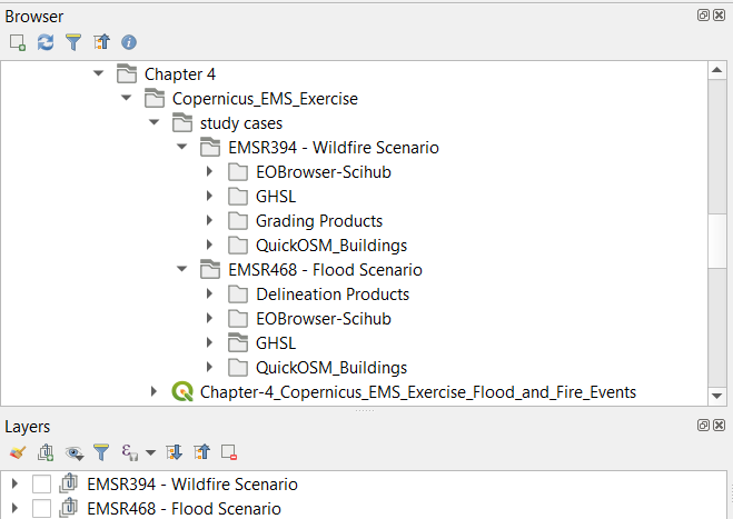
Fig. 4.2.1 QGIS project folders and layers structure
For the project we will make use of the Google Satellite base map which you can set though the “QuickMapServices” plugin. On the menu bar, go to Web (1) → QuickMapServices (2) → Google (3) → Google Satellite (4) . This will not only allow us to define a base map for our project, but also define the project Coordinate Reference System - CRS (in case this is the first added layer). The project CRS will be set to the EPSG:3857 – WGS 84 /Pseudo-Mercator.
Note
The EPSG:3857 , also known as Web Mercator projection, is a Spherical Mercator projection coordinate system. It is the standard projection used on web-based mapping programs.
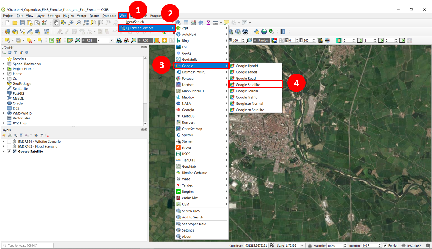
Fig. 4.2.2 Add the “Google Satellite” base map through the QuickMapServices
4.2.1. Flood Mapping and flood impact
- Overview
Flood mapping helps to estimate the flood extent on a large scale. It is an important tool during different phases of an emergency giving support to emergency activities, including recovery and rehabilitation, as well as the planning of prevention measures. In this practice, we will exploit flood maps in order to show the impact of the flood for a specific study case.
- Objective
The purpose of this practice is to guide you on assessing the exposure of a human settlement in a flood event.
- Disaster type: Flood
- Disaster Cycle Phase: Recovery and Reconstruction, Relief and Response
- Context
“Since the first hours of the 3rd of October 2020 an intense weather perturbation affected the North of Italy, with heavy rain and strong winds. Both red and orange alerts were issued by the regional and National Civil Protection. The greatest damages are reported in the Liguria region, and in the northern and western part of Piedmont region where the amount of the precipitation recorded exceeds the historical rate since 1958. The heavy rainfall has caused the overflow of several rivers and flooding of many areas. The overflow of the Sesia river in the Piedmont region caused interruption of roads, the collapse of a bridge and the flooding of several areas. Two deaths have also been reported.” (Copernicus EMS Rapid Mapping Activation: EMRS-468)
Sentinel-2 Imagery
- True colors band for the pre- and post event of the AOI.
Workflow
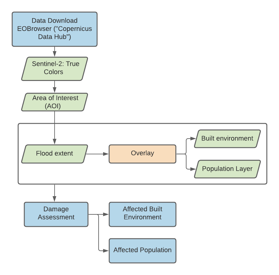
Fig. 4.2.1.1 Flood mapping exercise workflow
- Copernicus EMS - Rapid Mapping
Before starting to do the exercise, it is worth to mention how it was possible to identify the study case and the Area of Interest (AOI). For this purpose, we reviewed the Rapid Mapping list of activations published byt the Copernicus Emergency Management Service (CEMS) available in this link. In Fig. 4.2.1.2, you can find the different parameters set to query the activation of interest. Here, select Flood as event type (1) and Italy as the affected country (2). After the list of activations is updated with the defined parameters select the activation with the code EMSR468 (named Flood in Piedmont region, Italy) by clicking on its title (3).
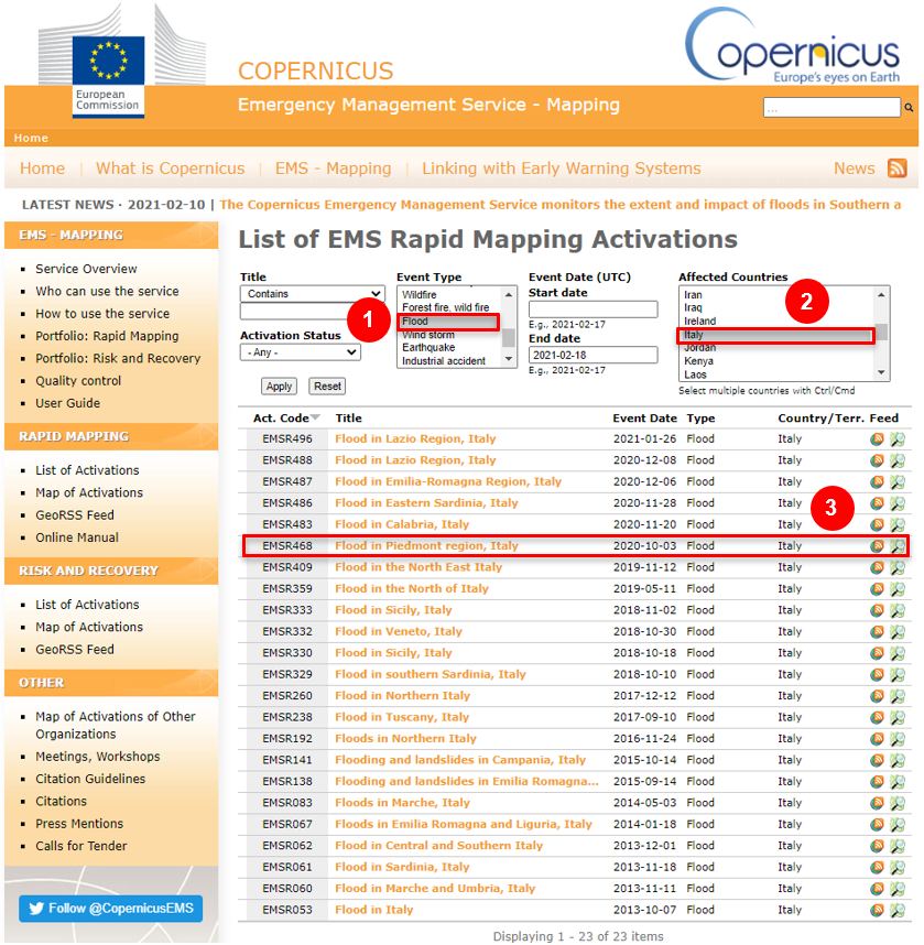
Fig. 4.2.1.2 Copernicus Rapid Mapping List of Activations - Flood events in Italy.
Note
In case you would like to search a different activation, there are other parameters which can help you to limit the query.
- Title: define logical operators (e.g.
equal,not equal,contains, etc. ) to search for specify keywords in the title of the activation. - Activation Status: define the current status of the activation.
Open(On-going) orclosed(Production finished) - Event type: select within a list of events the one of your interest.
- Event Start/End date: define a period to query the activations.
- Affected countries: Select one or multiple countries to query the activations. To select multiple elements from the list hold the ctrl key.
Once introduced the parameters the website execute the query for the matching activations. If for any reason the table does not update, click on the apply button.
For more information about the rapid mapping activities refer to the Online Manual for Rapid Mapping Products.
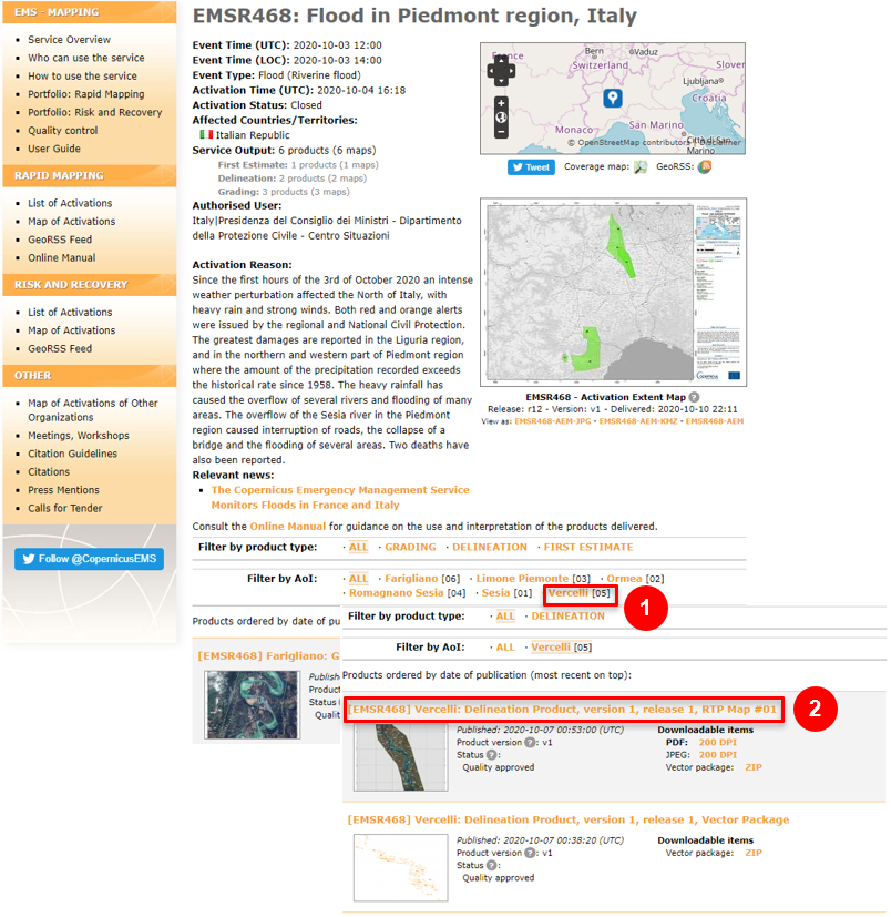
At this point, you should have reached the activation summary with details of the characteristics of the activation and the different products delivered for the activation (see Fig. 4.2.1.3). In this case, the activation involved multiple locations but for the exercise we will dedicate our attention to the delineation products in Vercelli. Here, there is the possibility to filter the products according to the typology and the AOI. Select Vercelli (1) as your AOI and [EMSR468] Vercelli: Delineation Product, version 1, release 1, RTP (2) as your product of interest.
Inside the product page, as seen in Fig. 4.2.1.4, you will have the option for:
- selecting the maps delivered by CEMS in PDF (1) and JPEG format
- downloading the CEMS vector layers produced for the delineation product by selecting the ZIP (2) file, accepting the disclaimers on the use of the products, and
download(3) the package.
Now, you can make use of the different layers produced for the AOI delineating the flooded area.
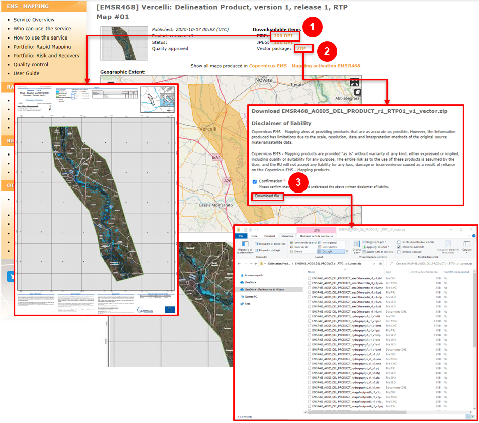
Fig. 4.2.1.4 Copernicus EMS Rapid Mapping, Delineation product, Flood in Piedmont Region, Italy. Vector Package Download (Delineation EMRS468).
- Data Download - EOBrowser
Next, we can proceed with the outline presented in Fig. 4.2.1.1.
Let us go to the EOBrowser platform to retrieve the Sentinel-2 optical satellite imagery for the AOI. Once that you have accessed your credentials you will have access not only to visualizing the Sentinel-Hub catalogue in the browser, but also the possibility to download the datasets.
Warning
This part of the practice imply that you have followed the lectures on “Sentinel Hub EO Browser” (https://gis4schools-rs.readthedocs.io/en/latest/rs_satelliteimages.html#) and that you are a registered “Sentinel-hub” user.
Now, we can define the querying parameters for our datasets of interest for the pre- and post-event of the flood event (see Fig. 4.2.1.5):
Use the search bar located at the top-right of you screen and search for
Vercelli, VC, Italia(1). Alternatively, you can move within the map canvas if you are familiar with the location, or you can upload a KML or GEOJSON file with the area of interest to identify the AOI.Data Source:
Sentinel-2(2)
Advanced Search:(3) →L2A (atmospherically corrected)(4)Time Range:
- Start date: 2020-09-20 (5)
- End date: 2020-10-03 (6)
After completely fill in the fields, click on the search (7) button to retrive the imagery.
Note
The Top of Atmosphere (TOA) corrections aim at separating the reflectance emitted for objects on the Earth’s surface from atmospheric disturbances that are part of the reflected energy recorded by the sensor. (https://www.un-spider.org/node/10958)
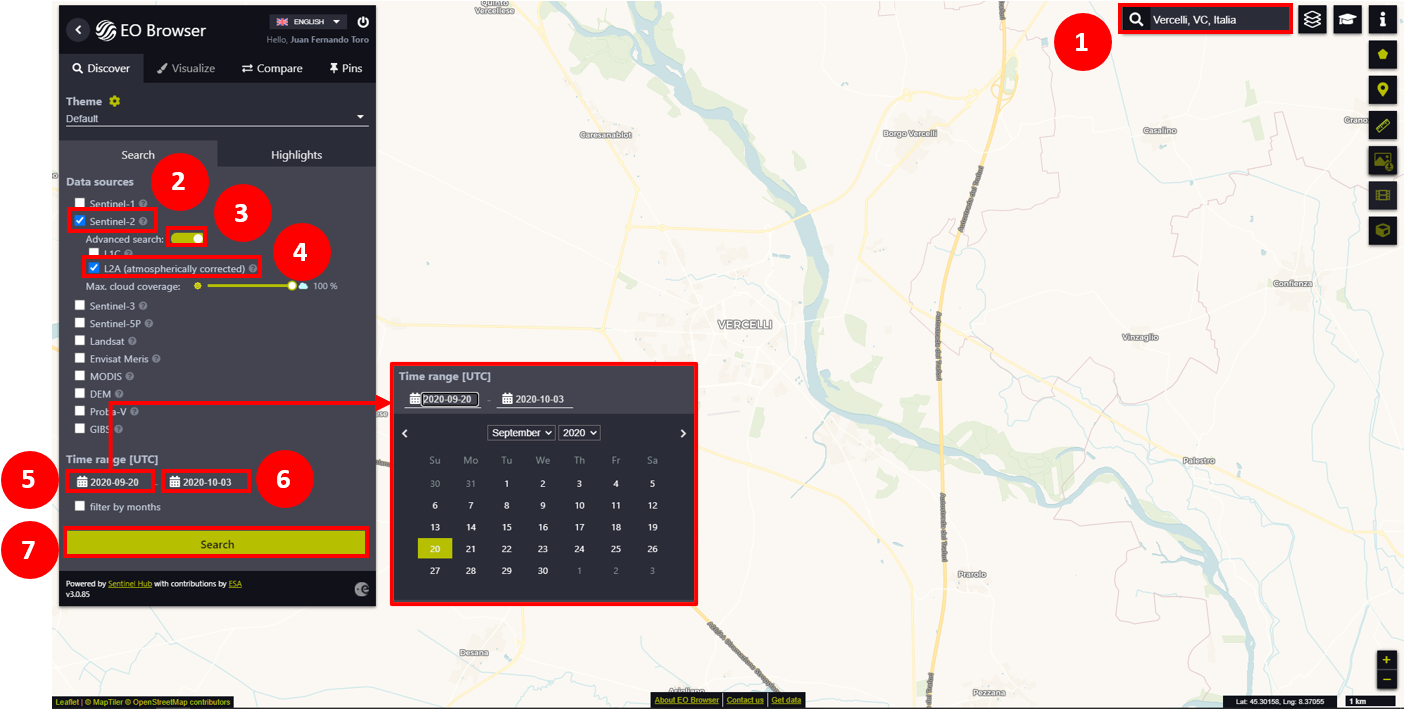
Fig. 4.2.1.5 EOBrowser viewer. CEMS Rapid Mapping activation EMRS468 Flood Event AOI.
On the left-side of the viewer, select the image for the September 28, 2020 by clicking on the visualize (1) button in Fig. 4.2.1.6. Notice that while hovering over the different available imagery the polygon representing the image coverage will change of color. This polygons visualization enables the possibility to observe that the imagery encloses the AOI.
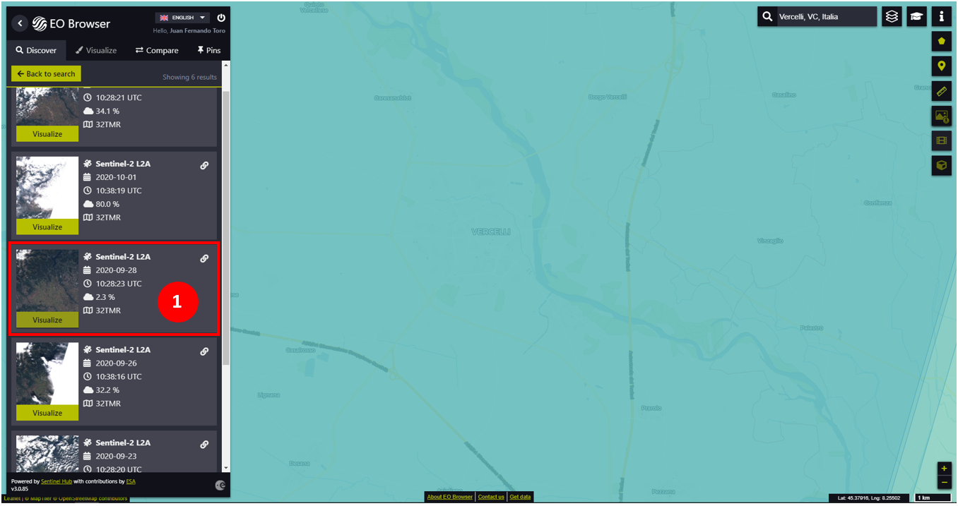
Fig. 4.2.1.6 EOBrowser viewer. Available imagery fulfilling the parameters.
Having selected the image, you will enable multiple functionalities to interact with the map and the dataset (see Fig. 4.2.1.7). Let us proceed to download the imagery. Click on the download function (4) to open the download window. Then, access the analytical (7) tab to define the data format and typology of your preference for downloading the data. In this case, input the following parameters to download the data:
- Image format:
TIFF (32-bit float)(8)- Image resolution:
HIGH(9)- Coordinate system:
WGS 84 (EPSG:4326)(10)- Layers:
True Color(11)
Then, click the Download (12) button, that will execute the download of the requested datasets. Each of the selected layer(s) are compressed into a ZIP file. By default the files are downloaded by the name of EO_Browser_images.zip.
Rename the file as EO_Browser_images_pre.zip. Move the file under the .\Copernicus_EMS_Exercise\study cases\EMSR468 - Flood Scenario\EOBrowser-Scihub.
Important
The downloaded images are relative to the current extent of the map viewer. When retrieving the data for a certain extent, avoid dragging or zooming the map view as it will change extent covered by the images.
Alternatively, you can draw within the map canvas if you are familiar with the location, or you can upload a KML or GEOJSON file with the area of interest to identify the AOI.
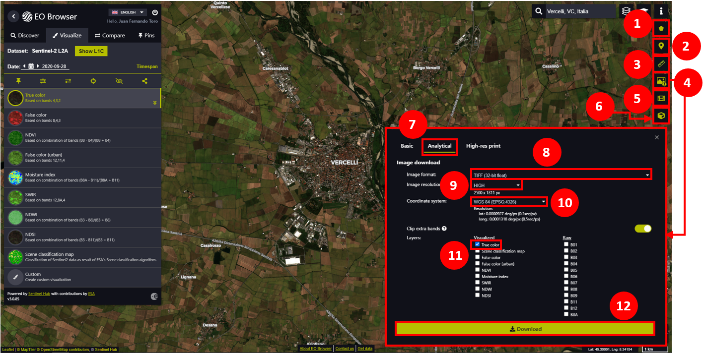
Fig. 4.2.1.7 EOBrowser viewer. Flood event area of interest data download.
Note
For more information about the functionalities provided by the satellite imagery viewer seen in Fig. 4.2.1.7, such as define an AOI (1), Mark a point of interest (2), Measure (3), Download image (4), Create time lapse animation (5) and Visualize terrain in 3d (6), visit the EOBrowser user-guide.
Fig. 4.2.1.8 present the pre- and post event imagery (atmospherically corrected) for the true colors of the imagery. Having imagery in different phases of the emergency allow to identify which is the hydrography of the AOI in normalcy with respect to the flooded areas. To query different images in time, EOBrowser provide two options to reach the imagery contained within the time span defined in previous steps. The first option is to return to the Discover (1) tab to reach the list of images and visualize a different image. And the second option, is to use the arrows presented next to the date to move backwards/forwards (2) in time to visualize the available imagery. Here, you will have the possibility to search suitable, cloud-free, imagery of your AOI for the later processing.
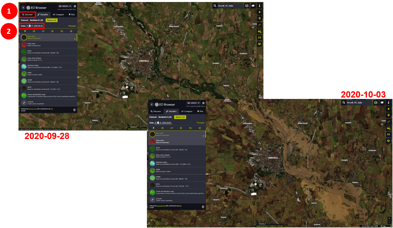
Fig. 4.2.1.8 EOBrowser viewer. Flood event pre- (2020-09-28) and post-event (2020-10-03) view.
Proceed to change the date until reaching October 3, 2020 (2020-10-03) to find the post event imagery. Repeat the previous steps presented in Fig. 4.2.1.7 to download the post-event dataset. Rename the downloaded ZIP file as EO_Browser_images_post.zip and move the file to the folder .\Copernicus_EMS_Exercise\study cases\EMSR468 - Flood Scenario\EOBrowser-Scihub.
- GHSL-POP
In this section, you will download the population datasets which will support the assessment of the exposure of the inhabitants of the AOI with respect to the flood event.
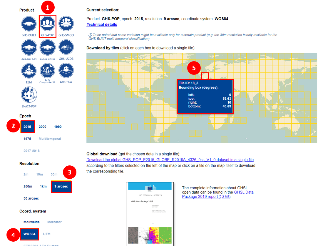
Fig. 4.2.1.9 GHSL-POP 2015 dataset. Tile 18_3 data download. https://ghsl.jrc.ec.europa.eu/ghs_pop2019.php
Here we will download the tiles of the GHSL-POP product, providing spatial distribution and density of population, detailed in section Other Useful Resources. Fig. 4.2.1.9 presents the steps required to download the population tile for the AOI. Select the following parameters relative to the population layer:
- Product:
GHS-POPlayer (1)- Epoch:
2015(2)- Resolution:
9_arcsec(3)- Coord. system:
WGS84(4)
After defining the parameters the tiles layer, click on the tile 18_3 (5) on the map viewer. The downloaded file will have the name GHS_POP_E2015_GLOBE_R2019A_4326_9ss_V1_0_18_3. The naming of the file summarize the set of parameters and the selected tile of the population layer.
Now, we can move to our desktop GIS to evaluate the impact of the flood by overlaying the different datasets retrived until this point.
Warning
The upcoming steps require to have followed:
- Sections 1.4. - 1.9. in chapter 1. Data visualization with QGIS.
- Section 2.3. Extending QGIS functionalities
- Section 2.5.5. Clip raster with a mask
- Section 3.4.1.8. Semi-Automatic classification Plugin.
- Evaluating the impact of the flood
This exercise will devote its attention to identifying the infrastructure (buildings) and population (GHS-POP layer) exposed within the flooded area.
In the next steps we will:
- Add the sentinel-2 pre- and post-event imagery
- Add the vector file concerning the AOI for the CEMS activation
- Add the GHSL-POP dataset
- Clip the GHSL-POP enclosed within the AOI
- Extract the building features within the AOI from OSM using the QuickOSM plugin
- Build the hazard map by combining the layers and defining different symbology
- Prepare a map composition of the hazard assessment
- Add the two images for the pre- and post-event from the paths and file names as specified below.
- Pre-event:
- Path:
.\Copernicus_EMS_Exercise\study cases\EMSR468 - Flood Scenario\EOBrowser-Scihub\EO_Browser_images_pre.zip- File name:
2020-09-28-00_00_2020-09-28-23_59_Sentinel-2_L1C_True_color.tiff
- Post-event:
- Path:
.\Copernicus_EMS_Exercise\study cases\EMSR468 - Flood Scenario\EOBrowser-Scihub\EO_Browser_images_post.zip- File name:
2020-10-03-00_00_2020-10-03-23_59_Sentinel-2_L1C_True_color.tiff.
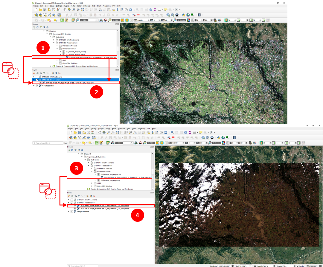
Fig. 4.2.1.10 EMSR468 Flood Event in Piedmont Region. Pre- and post event imagery.
Notice from Fig. 4.2.1.10 that the event imagery are represented with a different symbology. The symbology for both layers is assigned according to the ranges of values for each of the bands composing the true image colors. In this case, the presence of clouds in the post-event imagery force a wider range of values on the RGB bands which leads such contrast between the images symbology. Then, to compose the true colors in an equivalent way, we must set the same ranges of values of the RGB bands from the multiband symbology. To do so, first we must review the ranges of values for the RGB bands from each multiband image as presented in Fig. 4.2.1.11.
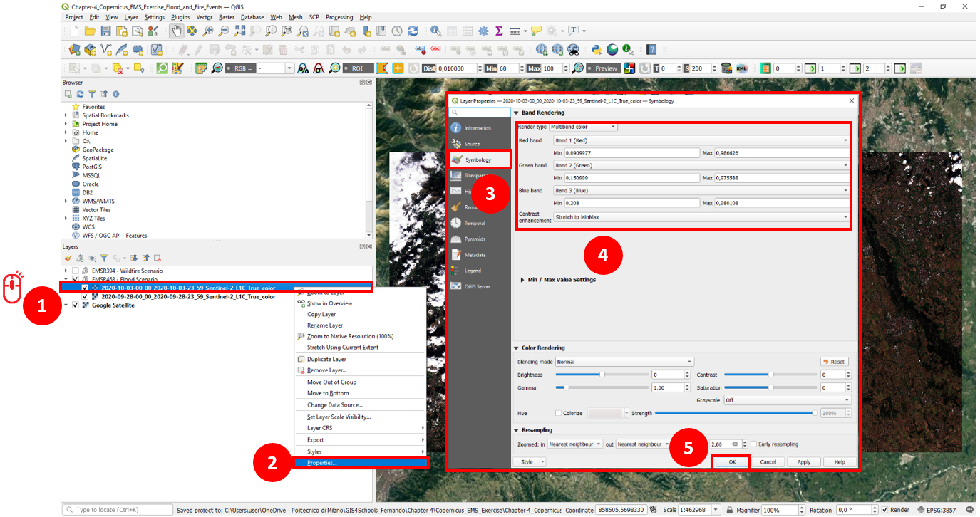
Fig. 4.2.1.11 Edit the RGB symbology for a multiband image.
To modify the values from the multiband symbology follow the steps in Fig. 4.2.1.11. Right-click on the layer to edit (1) → Properties... (2) → Symbology (3). Then, assign the values to the minimum and maximum values to the RGB bands presented in Table 4.2.1.1 (4). Finally, click on OK (5).
The values in the table comprise the minumum and maximum values contrasting the two images.
Follow the previous steps for both of the pre- and post event imagery.
| Band | Min | Max |
|---|---|---|
| Red | 0,0909977 | 0,986626 |
| Green | 0,143751 | 0,975588 |
| Blue | 0,193248 | 0,980108 |
Once the images share the same ranges of values for the RGB bands, the images should be displayed as seen in Fig. 4.2.1.12
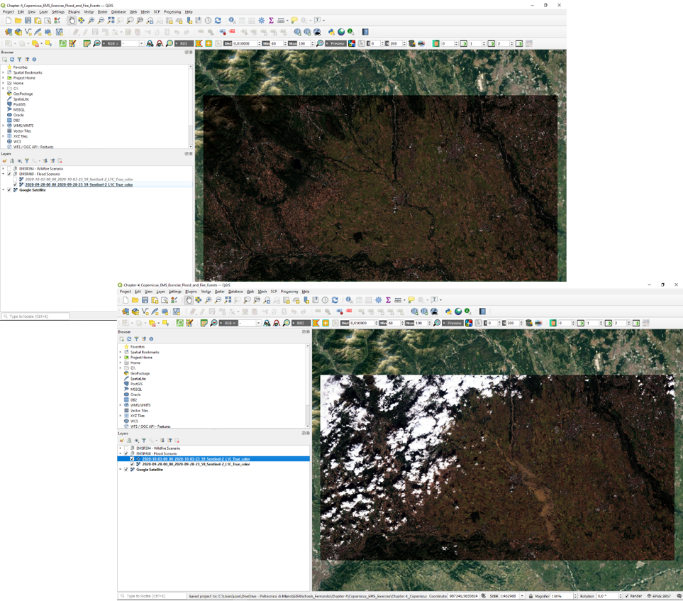
Fig. 4.2.1.12 Pre-event(top) and post-event(bottom) images sharing the same multiband symbology.
- Now, we will add the AOI layer provided within the delineation products downloaded from the CEMS service.
To add the new layer, on QGIS Browser, locate the path to the activation delineation products and expand the compressed file. The location and file to be added are:
- Path:
.\Copernicus_EMS_Exercise\study cases\EMSR468 - Flood Scenario\Delineation Products- File:
EMSR468_AOI05_DEL_PRODUCT_areaOfInterestA_r1_v1.json
After locating the file drag and drop the file inside the layer group for the flood activation (1) (see Fig. 4.2.1.13).
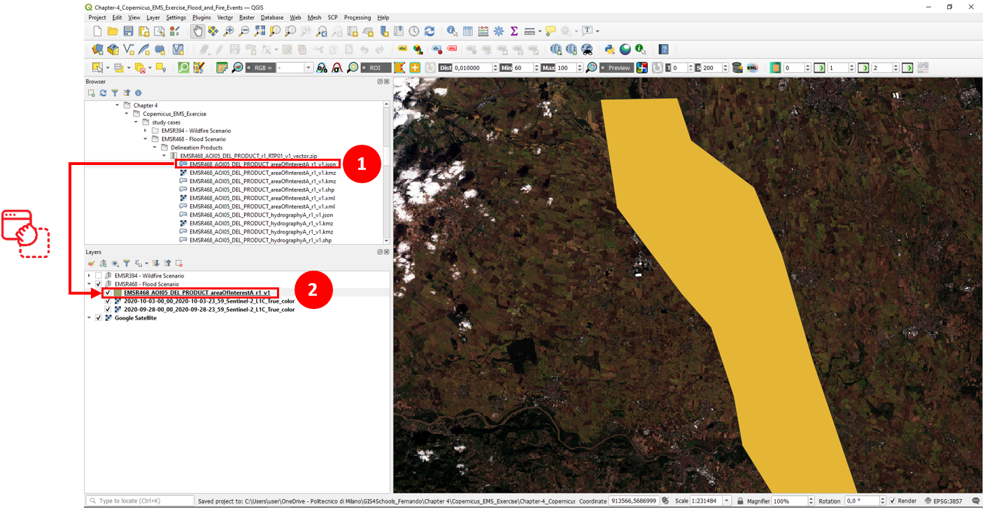
Fig. 4.2.1.13 EMSR468 activation - Flood event AOI.
Note
In the delineation products you will find different files and multiple formats for each. Each of the products is provided in KMZ, JSON, and SHP formats. In this case, the available products for the delineation activities for the flood are:
- Area of Interest: Identified area for assessing the flood extent.
- Hydrography: “Permanent” water bodies within the AOI.
- Image footprint: Polygon displaying the extent of the imagery used for the assessment.
- Observed event: Identified flooded area by the Rapid Mapping service.
- Transportation: Roads network within the AOI.
To contrast the flood extent delineated by the rapid mapping services, add inside your map the files of “hydrography” and “observed event”.
EMSR468_AOI05_DEL_PRODUCT_observedEventA_r1_v1.jsonEMSR468_AOI05_DEL_PRODUCT_hydrographyA_r1_v1.json
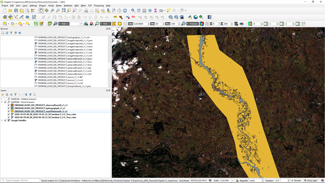
Fig. 4.2.1.14 EMSR468 activation - Delineated flood extent in the AOI.
Up to this point, with the current layers it is possible to compose a map of the impact of the flood (provided that we have the delineation products for this specific event). However, there are other different resources which can allow to carry out more complete analysis for the flooded area. 3. The next step is to add the currently available information concerning the population. For this purpose we will add the previously downloaded population tile from GHS-POP.
On your QGIS browser panel search for the following path:
- Path:
.\Copernicus_EMS_Exercise\study cases\EMSR468 - Flood Scenario\GHSL
Inside the folder you will find a compressed file with the name GHS_POP_E2015_GLOBE_R2019A_4326_9ss_V1_0_18_3.zip. Within the QGIS, expand the compressed file to find the GHS-POP raster file of the downloaded data.
- File Name:
GHS_POP_E2015_GLOBE_R2019A_4326_9ss_V1_0_18_3.tif
Click on the GHS-POP file (1) and drag and drop the dataset inside the group of the flood scenario (2) (see Fig. 4.2.1.15).
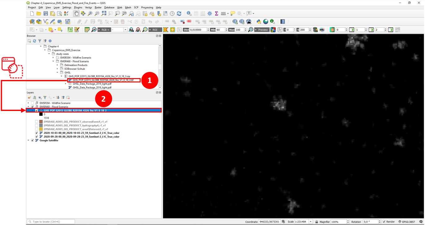
Fig. 4.2.1.15 EMSR468 activation - add GHS-POP 2015 layer tile 18_3.
- Extract the population data enclosed by the area of interest.
The next step is then to narrow down the information we have with respect to the population for the AOI. To achieve this, we will make use of the “clip raster with mask” processing tool. In Fig. 4.2.1.16 are detailed the steps to crop the GHS-POP raster. On the menu bar, select Raster (1) → Extraction (2) → Clip Raster by Mask Layer (3). On the “Clip Raster by Mask Layer” window, input the following parameters:
- Input Layer:
GHS_POP_E2015_GLOBE_R2019A_4326_9ss_V1_0_18_3 [EPSG:4326](4)- Mask Layer:
EMSR468_AOI05_DEL_PRODUCT_areaOfInterestA_r1_v1(5)
Scroll-down on the window (6) until finding the “Clip (mask)” option → ... (7) → Save to File ... (8) . Reach the path to the location of your GHS-POP dataset and save the clipped file as GHS_POP_E2015_GLOBE_R2019A_4326_CLIP. Activate the Open output file after running algorithm (9) to add the layer in your project after executing the command by clicking on Run (10).
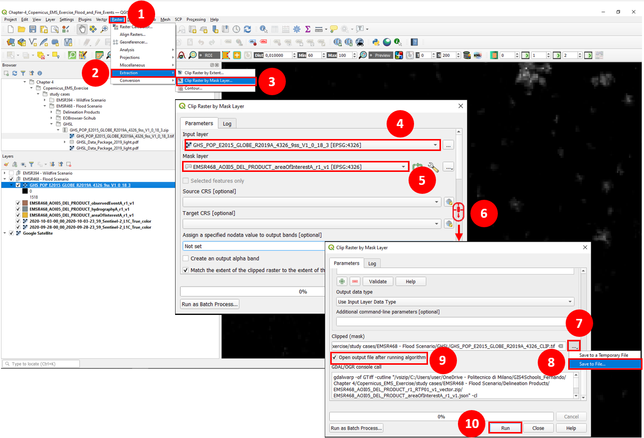
Fig. 4.2.1.16 EMSR468 activation - clip GHS-POP 2015 within the AOI.
Fig. 4.2.1.17 display the output of the cropped layer of the GHS-POP tile.
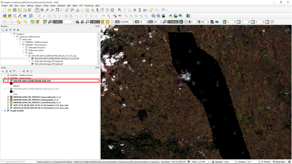
Fig. 4.2.1.17 EMSR468 activation - clipped GHS-POP 2015 within the AOI.
The maps should be as clear and insightfull as possible. For this, assigning proper symbologies to the layers is a must. Fig. 4.2.1.17, details the procedure to create a symbology which highlights the human settlements and defines suitable labels to represent the count of people per pixel in the layer.
To modify the symbology from the clipped layer, right-click on the GHS_POP_E2015_GLOBE_R2019A_4326_CLIP layer (1) → Properties ... and in the Symbology tab select the following parameters:
- Render type:
Singleband pseudocolor(3)- Interpolation:
Discrete(4)- Color ramp: Choose a fitting color ramp (5)
- Label precision:
0(6)- Mode:
Continuous(7)
Apply the symbology by clicking on Classify (9) → OK. The layer should be now visualized as seen in :numref:4.2.1.19.
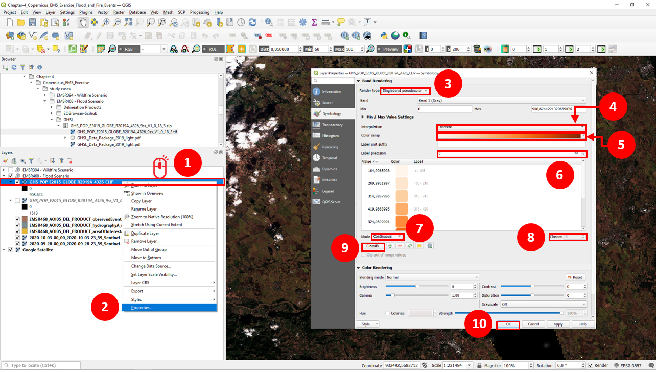
Fig. 4.2.1.18 EMSR468 activation - modify clipped GHS-POP 2015 symbology.
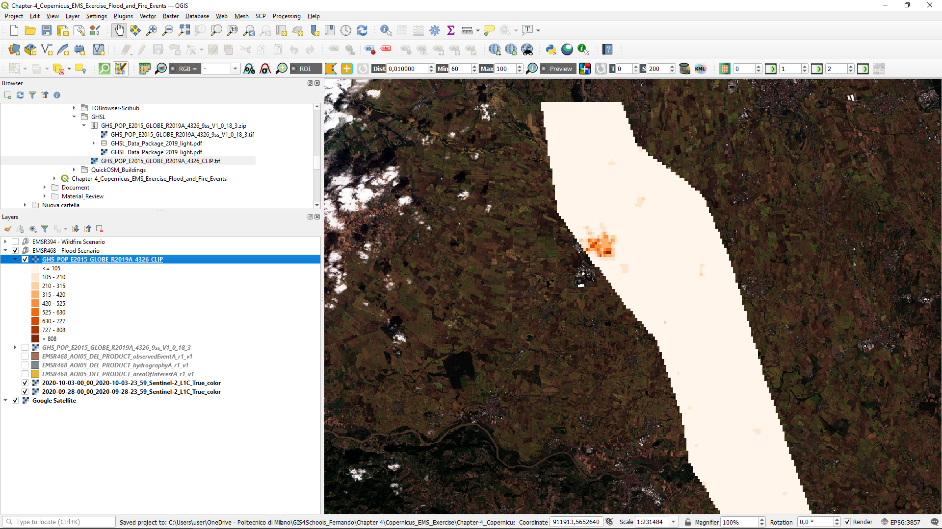
Fig. 4.2.1.19 EMSR468 activation - GHS-POP 2015 for the AOI.
Important
The population exposure may as well be performed by using more detailed datasets from local census or other sources.
- Query the OSM buildings features using the QuickOSM plugin.
For the extraction of the OSM features follow the instruction in Fig. 4.2.1.19. On the menu bar, select Vector (1) → QuickOSM (2) → QuickOSM... (3), and enter the Symbology tab:
- Key:
building(4) - Value:
yes(5) - In:
Layer Extent(6) →EMSR468_AOI05_DEL_PRODUCT_areaOfInterestA_r1_v1(7)
Here, we will open the Advanced (8) option to define a folder to store the data. Here, click on ... (9) and select the location:
- Path:
.\Chapter 4\Copernicus_EMS_Exercise\study cases\EMSR468 - Flood Scenario\QuickOSM_Buildings
And proceed to Run query (10). After the process is executed, the OSM features with the key-value pairs, building-yes, have been added to the map (See Fig. 4.2.1.20).
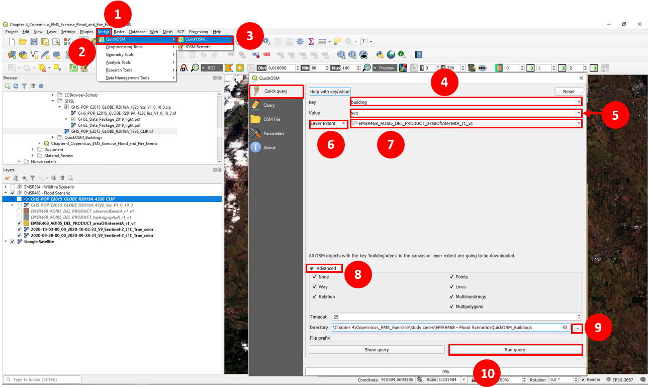
Fig. 4.2.1.20 EMSR468 activation - QuickOSM building features (yes) query.
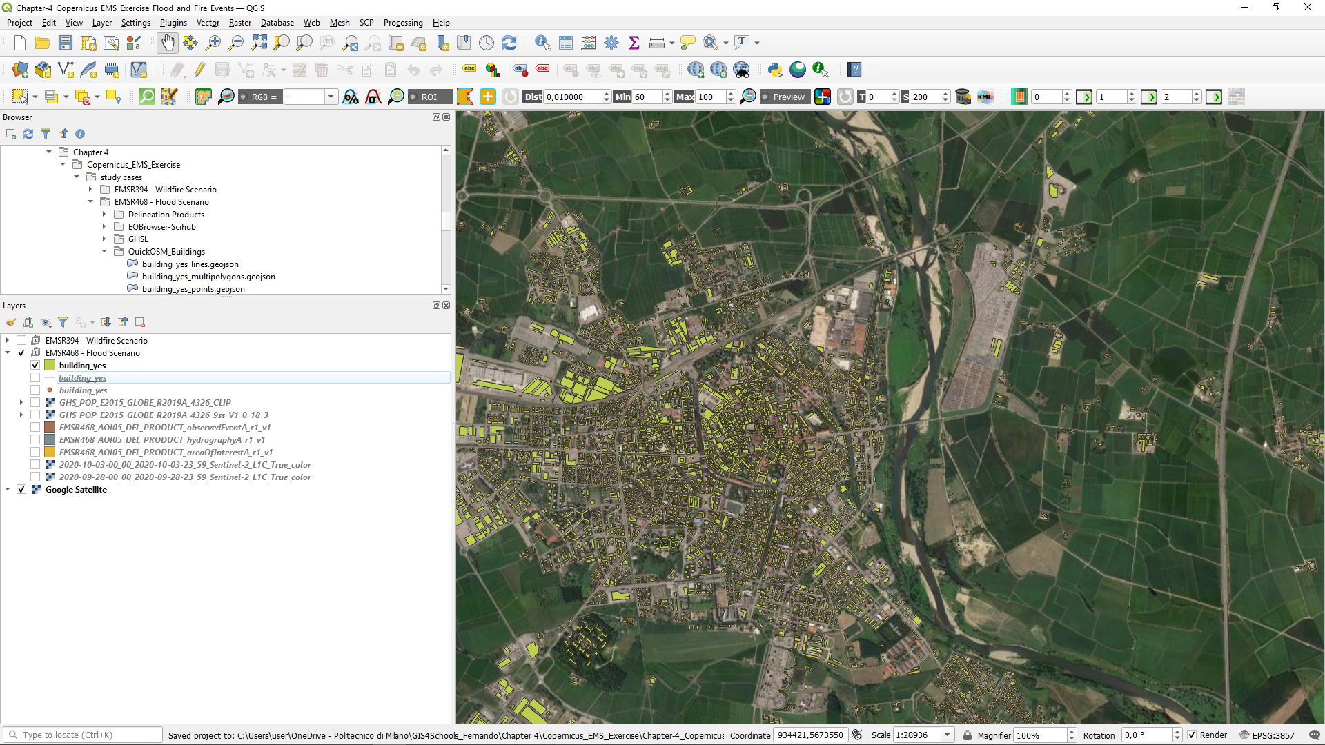
Fig. 4.2.1.21 EMSR468 activation - QuickOSM building features.
- Build the impact assessment map by combining the layers and defining different symbologies
As stated previously, crucial asset for hazard mapping is the representation of information. In Fig. 4.2.1.21, the layers symbology has been modified to provided a more intuitive layout with respect to the flood event. First by distinguishing the permanent water bodies with respect to the flood plain. Second, by providing contrasting colors to the buildings and population. Another point which can improve the layout of your map is to add transparency and overlay to the layers.
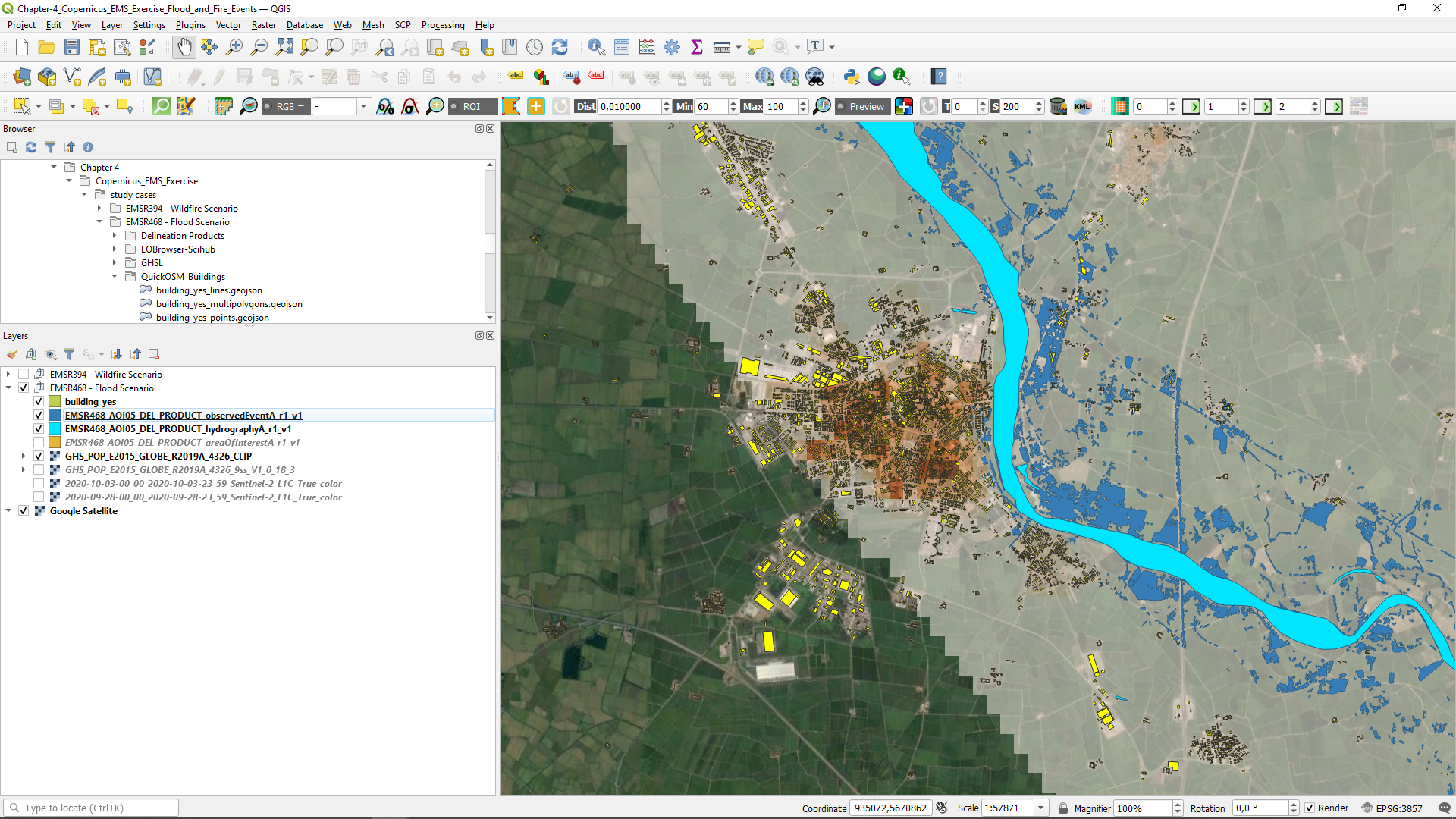
Fig. 4.2.1.22 EMSR468 activation - Editing of the layers visualization.
The flood mapping activities enable the identification of the affected infrastructure. Let us now target the buildings which have been affected by the flood. First, provide the building layers attribute table with a field that states if they are within the flooded areas (see Fig. 4.2.1.23). Open the attribute layer for the building layer and create a new field. Right-click on the layer (1) and select the Open Attribute Table (2). Field Calculator (3) → Create new field (4) → with an output field name impact (5) and output field type Text (string) (6) and an output field length of 15 (7). Then, in the expression box assign the value 'not affected' (8) which will be the default value in case the building is not inside the mapped flooded areas. At last, click on OK (9).
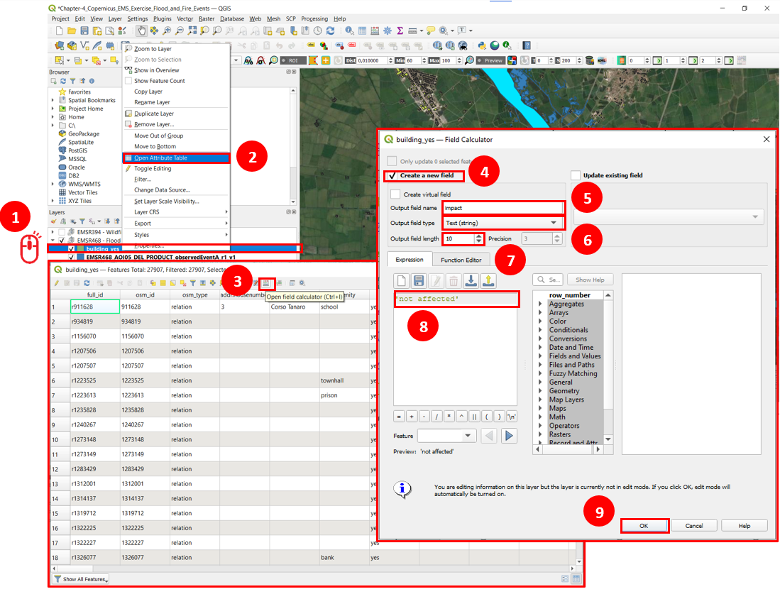
Fig. 4.2.1.23 Add a field to assign the impact categories to the building features.
Note
Currently, the buildings layer editing mode is enabled. Beware of any modification of the layer because they will be saved once the editing mode is disabled. Be careful no to modify any of the contents of the table while the editing is active.
It could be the case that in later scenarios the flood plain can extend in wider areas. Let us compose a scenario in which the flood extent is 50m larger with respect to this event. To build this scenario we will make use of the buffer tool (see 2.4.6. Geoprocessing tools for vector data: buffer). To make use of the buffer tool, first we need to set an appropriate cartographic representation for the flood extent layer to be able to carry out the offset of the layer (the buffer/offset units are linked to the CRS of the layer). For this reason, we need to reproject the layer into projected coordinate system. To reproject a layer into a different CRS (see Fig. 4.2.2.24), select Vector (1) → Data Management Tools (2) → Reproject Layer … (3). Here, the Input layer is EMSR468_AOI05_DEL_PRODUCT_observedEventA_r1_v1 EPSG:4326 (4) and the target CRS is the Project CRS: EPSG:3857 – WGS 84 /Pseudo-Mercator (5) → Run (6). The created layer will have the name Reprojected (see Fig. 4.2.2.25).
Note
When selecting a projection consider the purpose of your map. In case you would like to present a reference map of the globe, you may prefer to find a balance between shape and area distortions. On the other hand, if your map has a specific purpose you may prefer to avoid large distortions in shape or area. See section 1.2.1. Projections
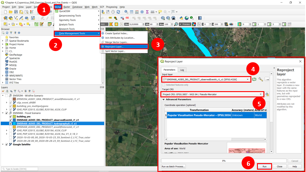
Fig. 4.2.1.24 Reproject the observed event layer.
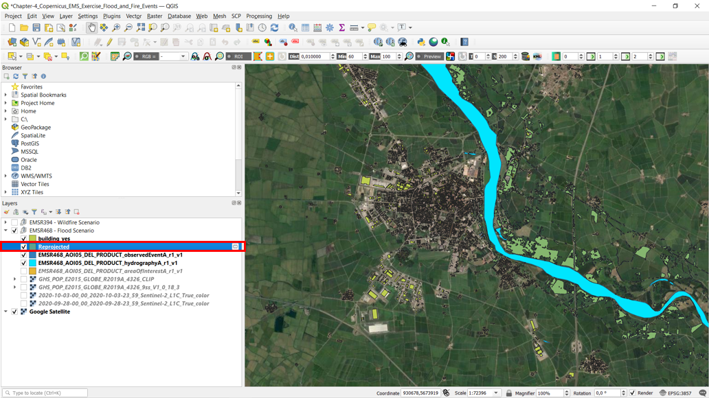
Fig. 4.2.1.25 Reprojected observed event layer, EPSG:3857.
Let us save the temporary file of the reprojected layer. Fig. 4.2.2.26 present the steps for saving the new layer. Right-click on the layer named Reprojected (1) → Export (2) → Save Feature As … (3). On the appearing window, select the format as ESRI Shapefile (4). Define the path and name to the file .\Copernicus_EMS_Exercise\study cases\EMSR468 - Flood Scenario\Delineation Products\flood_scenario.shp (5). Set the Coordinate Reference System as EPSG:3857 – WGS84 / Pseudo-Mercator (6). Click on OK. The layer should be added directly into the project if the Add saved file to map is enabled (if not, add the layer from the location set at step (5)).
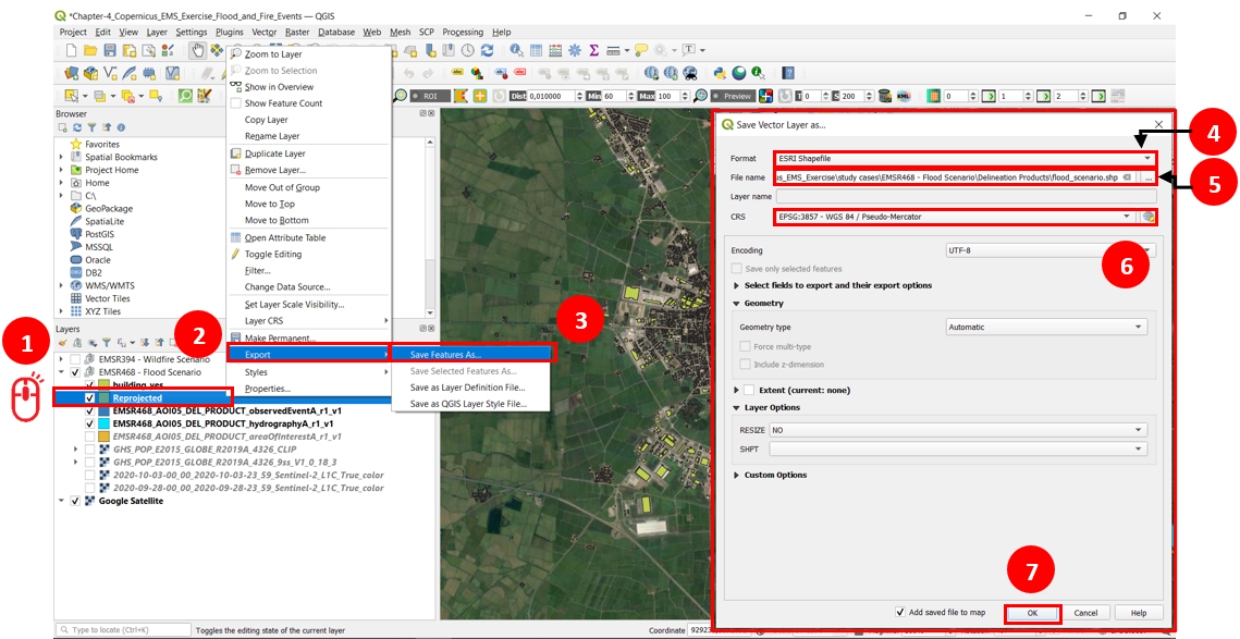
Fig. 4.2.1.26 Save the temporary reprojected layer in the exercise working folders.
Note
In some cases, the use of geoprocessing tools such as “select by location” (see section 2.4.2. Attribute table: selection, editing and field calculator.) can lead to the following error message(s): “Feature (X) has invalid geometry” and/or “Execution failed after X.X seconds”. To solve this, you may need to fix the geometry or change the Processing setting to the “Ignore invalid input features” option. To address this issue, create buffer of 0 m width for the flooded areas layer (later in the exercise we will create a 50m buffer). In this way we fixed the invalid geometry, and we will use flood_scenario_fixed layer for future selections (see Fig. 4.2.2.27).
The next step considers creating a buffer around the flooded area to fix some issues concerning the features included in the Observed event layer as shown in Fig. 4.2.2.27. On the menu bar, select Vector (1) → Geoprocessing Tools (2) → Buffer (3). In the new window, select flood_scenario as the input layer (4). Assign an offset of the polygon of 0 (5) meters (6). Define the output path file and name .\Copernicus_EMS_Exercise\study cases\EMSR468 - Flood Scenario\Delineation Products\flood_scenario_fixed.shp (7). Activate the Enable output file after running algorithm. Click on Run.
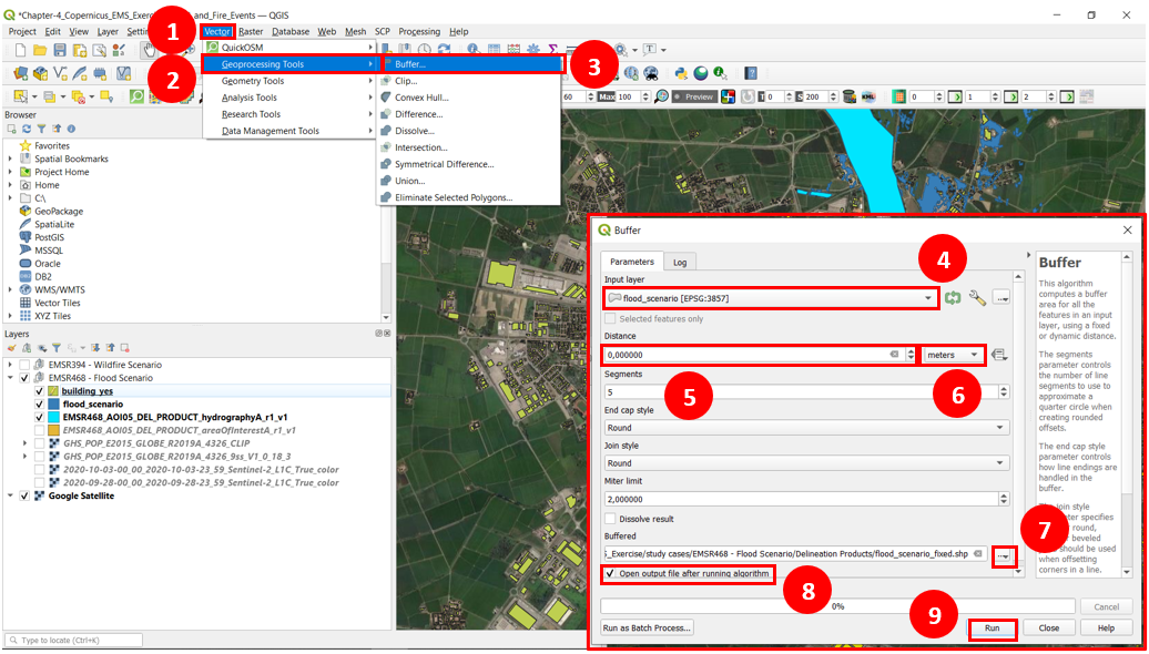
Fig. 4.2.1.27 Perform a 0m buffer around the flood event to correct possible feature errors.
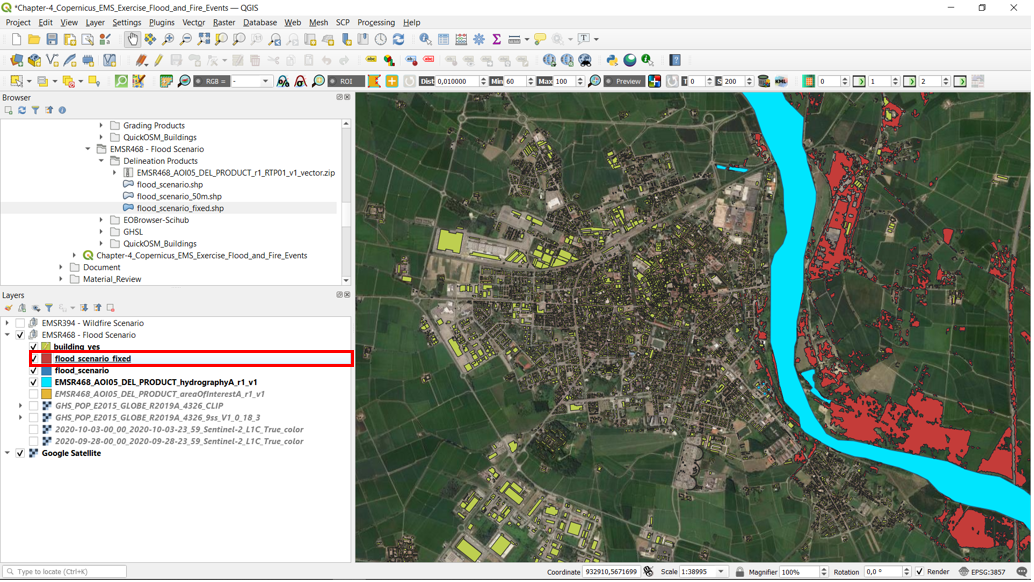
Fig. 4.2.1.28 “Fixed” flood extent, 0m buffer around the flood event to correct possible feature errors.
Using the field created inside the building layer we can identify the buildings which have been affected by the flood intersecting the layers. Here, an approach is to select the features from one layer depending on another. On the menu bar, select Vector (1) → Research Tools (2) → Select by Location … (3). In the “Select by Location” window, choose the options as follows:
- Select features from:
building_ yes [EPSG:4326](4)- Where the features (geometric predicate):
intersect(5)- By comparing the features from:
flood_scenario_fixed[EPSG:3857](6)
Having set the parameters, execute the function by clicking on Run (7).
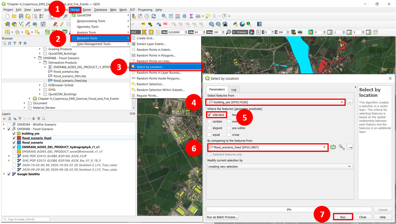
Fig. 4.2.1.29 Select building features located within the flooded extent.
Once selected the building laying inside of the flooded areas it is possible to provide a suitable value on the impact field of the building_yes layer. Open the building_yes attribute table. Notice that the selected features are highlighted in blue. Click on the Field Calculator icon (1). Enable the option of Only update *n* selected features (2). Check the Update existing field (3) option. Define the field to be modified impact (4). Set the value to assign in the field at the expression box (here assign a string defined as 'flooded' (5)). Click on OK to execute the operation (6). After the changes have been applied you will notice the changes as presented in (7). Notice that the attribute table remarks on the top of its window the number of selected features from the layer. In this case, we have that 7 building are located inside the observed event flood extent.
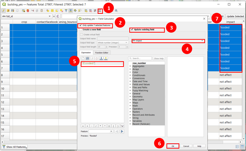
Fig. 4.2.1.30 Assign the “flooded” impact category to the buildings within the observed flooded area.
Next, we will replicate the steps to produce the flood_scenario_fixed layer, this time to make a 50 m buffer from the flooded area. In this case the buffer will model a scenario of a layer flood event. The scenario is going to indicate the buildings which could be in a flooded area. When the building in this specific scenario have been identified, the impact field on the building layer will take the value 'possible flood'.
Make a buffer of 50 meters around the flooded area following the steps presented in Fig. 4.2.1.31. This new buffer will be named flood_scenario_50m. The shapefile will be stored in the path and file name .\Copernicus_EMS_Exercise\study cases\EMSR468 - Flood Scenario\Delineation Products\flood_scenario_50m.shp. Fig. 4.2.1.32 presents the output layer from the buffer.
Note
It is important to remark that this is a simplified exercise to provide an alternative flood scenario. This scenario does not model the water flow inside the AOI in case of a flood event. Rigorous flood modelling consider the terrain geometry, land coverage, soil composition and other parameters.
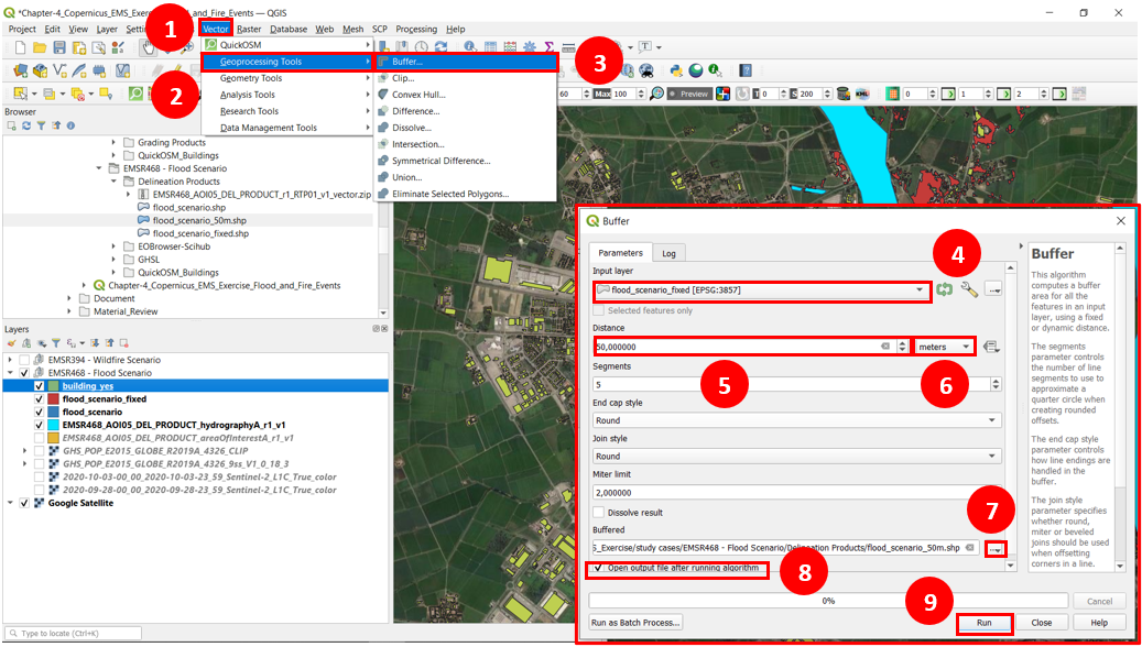
Fig. 4.2.1.31 Perform a 50m buffer that represents a larger flood extent scenario.
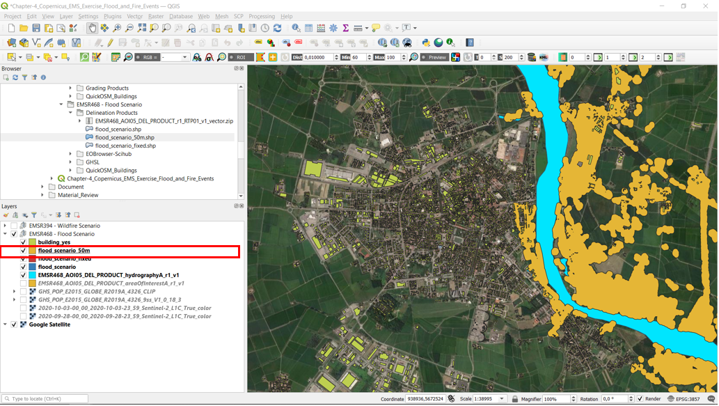
Fig. 4.2.1.32 “possible flood” scenario, 50m buffer around the flood event.
Now, it is possible to identify the buildings located inside the “possible flood” scenario. To do so, follow the steps presented in Fig. 4.2.1.33.
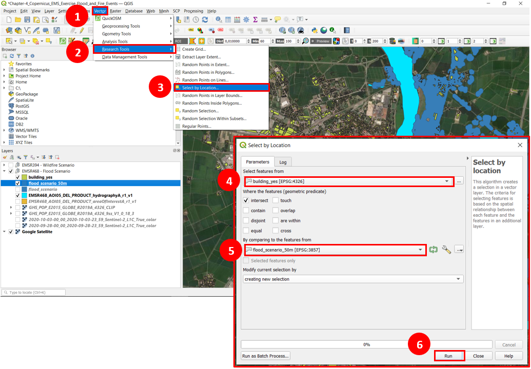
Fig. 4.2.1.33 Select building features located within the “possible flood” scenario flooded extent.
Once the buildings located inside the “possible flood” scenario have been selected, proceed to open the attribute table for the building_yes layer and follow the steps on Fig. 4.2.1.34. For this selected features a value of 'possible flood' will be assigned to the impact category.
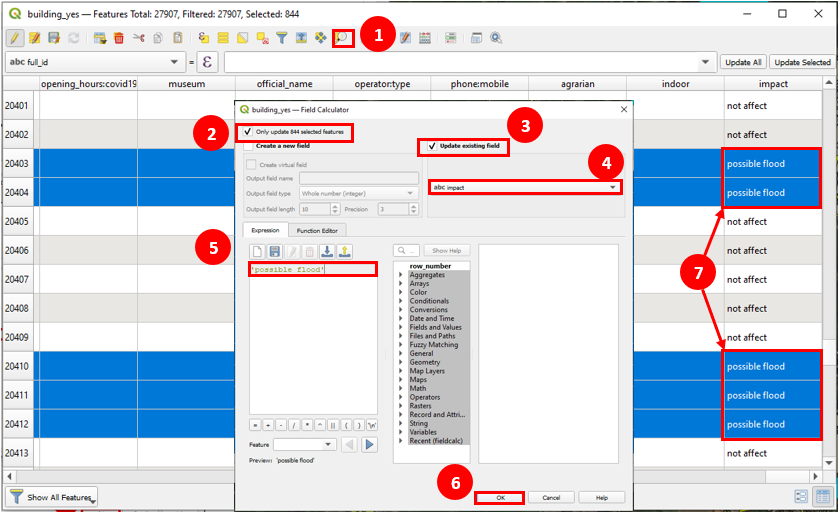
Fig. 4.2.1.34 Assign the “flooded” impact category to the buildings within the observed flooded area.
Until March 01st, 2021 there have been mapped a total of 27 buildings, from which 7 have been affected during the flood according to the delineation map and 844 building were nearby the flooded ares so they should be monitored.
Note
The results may vary, consider that the OSM team is actively working on and improving their datasets.
Now that we have assessed the impact on the buildings, we can provide a symbology based on the categories defined by the expected impact according to the defined scenarios.
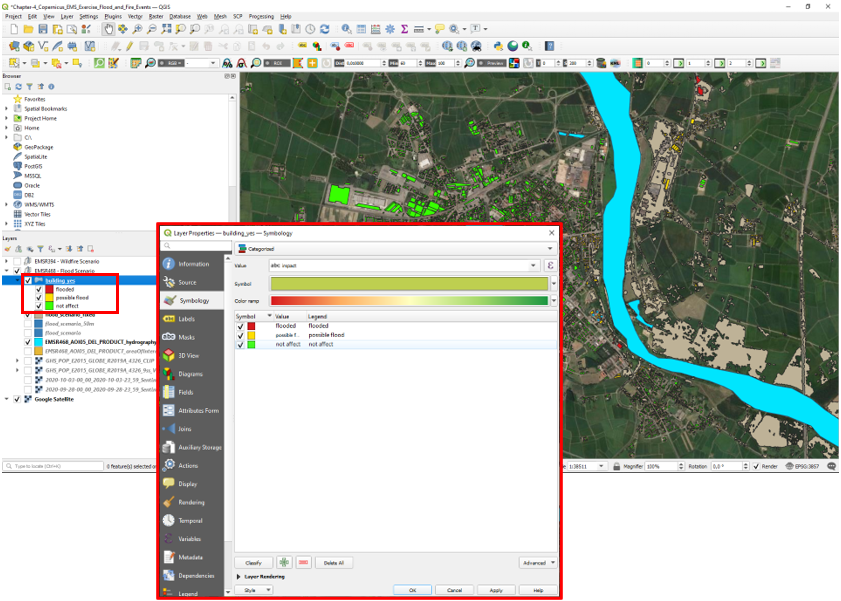
Fig. 4.2.1.35 Building features symbology based on the AOI.
It is possible to assess the count of buildings inside an impact class by selecting the features using the impact field (see Fig. 4.2.1.36).
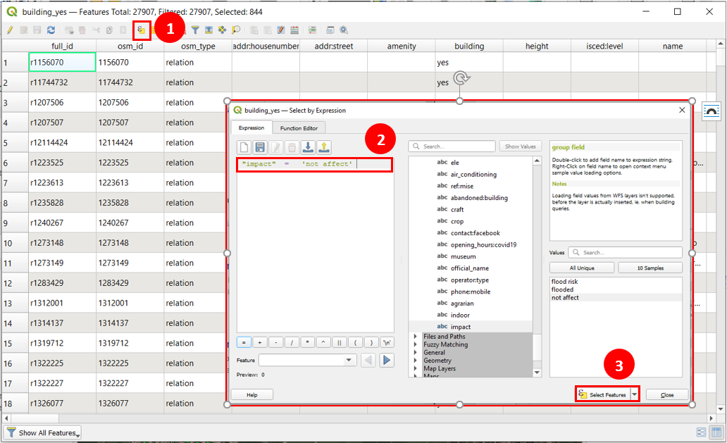
Fig. 4.2.1.36 Identify the buildings count by the impact field classification.
- Prepare a map composition of the flood impact
To set up your map composition, start by creating a new layout (see Fig. 4.2.1.37). On the menu bar select File → New Print Layout.... Give a name to your layout.
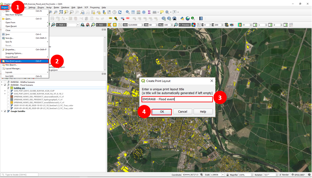
Fig. 4.2.1.37 EMSR468 activation - Layout for the hazard event.
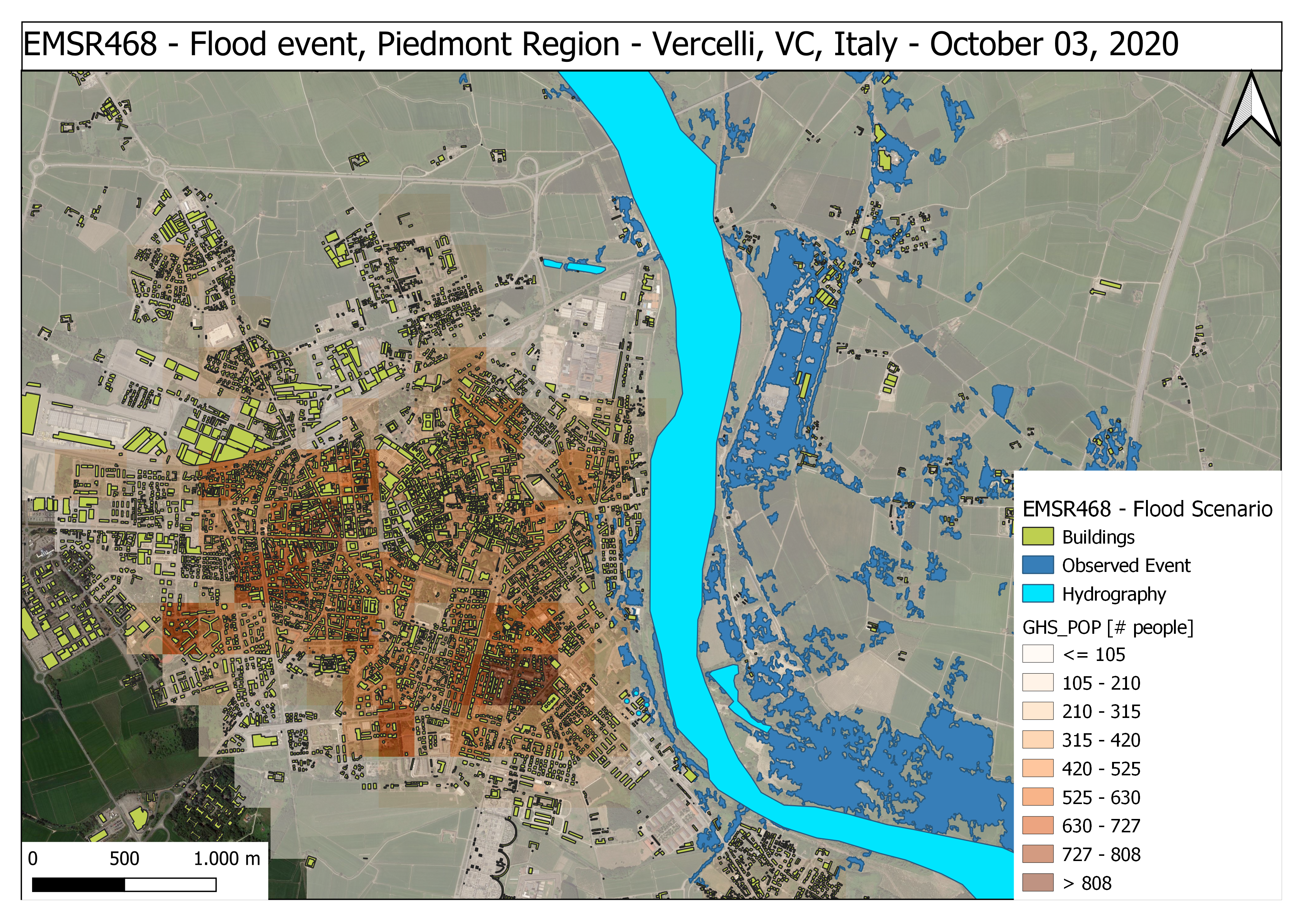
Fig. 4.2.1.38 EMSR468 activation - Flood impact map.
4.2.2. Fire Mapping
In this section we will dedicate our attention on the processing of Sentinel-2 satellite imagery to assess the damage from a fire event in the vicinity of an urban area.
- Overview
A wildfire is a rapidly spreading fire that also occur in woodland areas. Annual dry seasons or drought provide an ideal environment for biomass presence and dry conditions to combine. Ignition sources for wildfires can relate to natural events, such as lightning strikes or lava flow, unfortunately, they can also be man-made, resulting from the burning of debris, unattended campfires and intentional arson.
Wildfires can result in the loss of human life, wildlife, and impact directly, or indirectly, different ecological processes due to the removal of the vegetation layer. Therefore, it is essential the assessment of the severity of the impacted areas. This practice aims at assessing an affected area using remote sensing tools. The methodology will benefit from the use of the open satellite imagery published at the Copernicus Sci-Hub. Here, using Sentinel-2 imagery, you will model the severity of a wildfire in the Campania Region in Italy (in the vicinity of Sarno municipality). The severity assessment considers the comparison of pre- and post-event imagery by computing the Normalized Burnt Ratio (NBR) on each scenario.
Burnt severity data and maps can aid the development of emergency rehabilitation and restoration plans, post-fire. The proposed methodology is recommended for assessing the burn severity of large areas affected by wildfires.
- Objective
The purpose of this practice is to guide you on assessing the post-fire burned areas.
- Disaster type: Wildfire
- Disaster Cycle Phase: Recovery and Reconstruction, Relief and Response
- Context
“On 15/09/2019, a forest fire affected the municipality of Sarno (Salerno) in Italy, in the area of the Monte Saretto. The fire spread over the mountain behind the town of Sarno and for this reason almost 200 people have been evacuated. After a first analysis of the event, over 90% of the Sarno pine forest has been affected.” (CEMS Rapid Mapping Activation: EMRS-394)
The practice makes use of Sentinel-2 imagery.
For burn severity monitoring we will make use of Sentinel-2 Near Infrared (NIR) and Shortwave Infrared (SWI) bands. These bands have a spatial resolution of 20m.
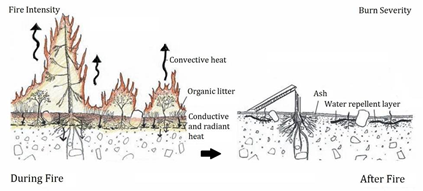
Fig. 4.2.2.1 –Illustration of fire intensity versus burn severity (Source: US Forest Service)
A measurement to highlight burnt areas is the Normalized Burnt Ratio (NBR), which tries to identify the effects of a fire in an area (after the combustion process). The NBR is an index designed to expose burnt areas in large fire zones.
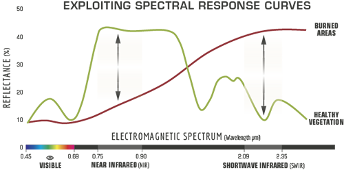
Fig. 4.2.2.2 –Comparison of the spectral response of healthy vegetation and burned areas (Source: US Forest Service)
The healthy vegetation shows a high reflectance in the NIR, and a low reflectance in the SWIR portion of the spectrum. On the other hand, there is the opposite behaviour in burnt areas. The NBR benefits from this difference in the spectrum to highlight a burnt area through the following relationship.
When the NBR value is high it indicates a healthy vegetation. While low NBR values indicate bare ground and recently burnt areas. Non-burnt areas area generally attributed a value of zero.
The difference between the pre-fire and post-fire NBR can be used to estimate the severity of the burnt area. This measurement is known as the Burn Severity. Higher values of this estimation indicate more severely damaged vegetation.
Burn Severity values can vary from case to case, and so, if possible, interpretation in specific instances should also be carried out through field assessment; in order to obtain the best results. However, the United States Geological Survey (USGS) proposed a classification table to interpret the burn severity presented in Table 4.2.2.1.
| USGS dNBR classification (Value <= dNBR) | HEX Color | Label (Severity Level) |
|---|---|---|
| -0.1 | #29BD2E | Unburned |
| 0.27 | #FFDE00 | Low Severity |
| 0.44 | #FF9100 | Moderate-Low Severity |
| 0.66 | #E3003B | Moderate-High Severity |
| 1.3 | #9D00C4 | High Severity |
Warning
The dNBR values may differ from case to case, so it is required to preform in field assessments for better results of the classification. Table 4.2.2.1 is a proposed classification provided by the United States Geological Survey (USGS). Click here for more information on the dNBR estimates.
Important
For a better understanding on the topic of exploiting the spectral signature for Earth Observation and environmental monitoring, please refer to sections:
- 3.2.1 The spectral signature
- 3.2.2 Spectral indices for environmental monitoring
- Sentinel-2 Imagery
The Sentinel-2 imagery required to develop this practice is:
- NIR and SWIR images for Sentinel-2 are the bands 8A and 12, correspondingly.
- The pre-event imagery was retrieved for the 03/09/2020.
- The post-event imagery was retrieved for the 14/09/2020.
- Workflow
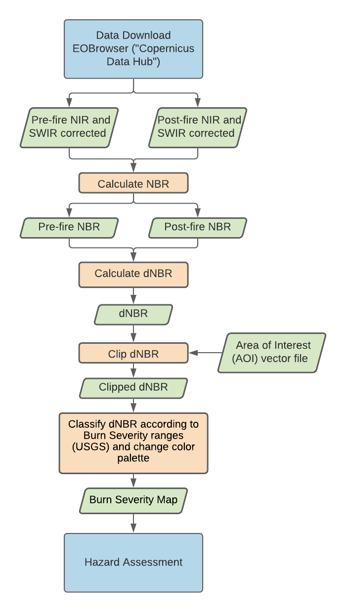
Fig. 4.2.2.3 –Fire mapping exercise workflow
- Copernicus EMS - Rapid Mapping
This exercise dedicates its attention to a wildfire event in Italy that took place in the vicinity of the city of Sarno (Campania Region).
Go to the CEMS - Rapid Mapping list of activations and input the querying parameters as defined in Fig. 4.2.2.4. Select the event type Wildfire (1) and Italy (2) as the affected country. When the table of activations has updated with the defined parameters search for the activation EMSR394. Click on the title of the activation to reach the page of the activation summary.
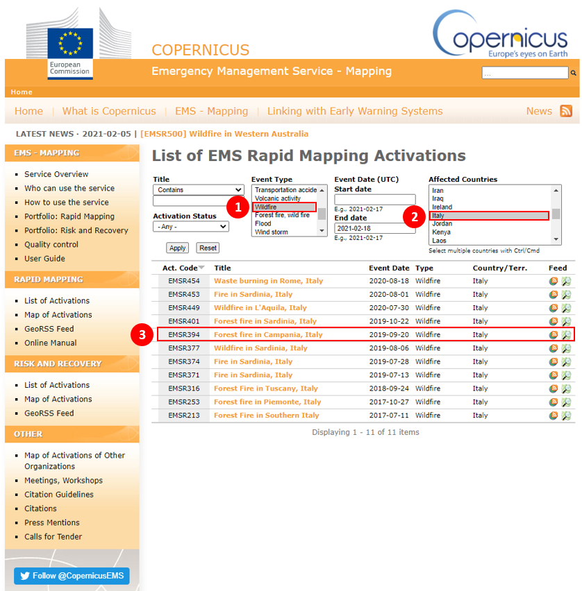
Fig. 4.2.2.4 –Copernicus Rapid Mapping List of Activations - Wildfire events in Italy
In the activation page, see Fig. 4.2.2.5, select the grading product with naming Sarno: Grading Product, version 1, release 1, RTP Map #01 (1).
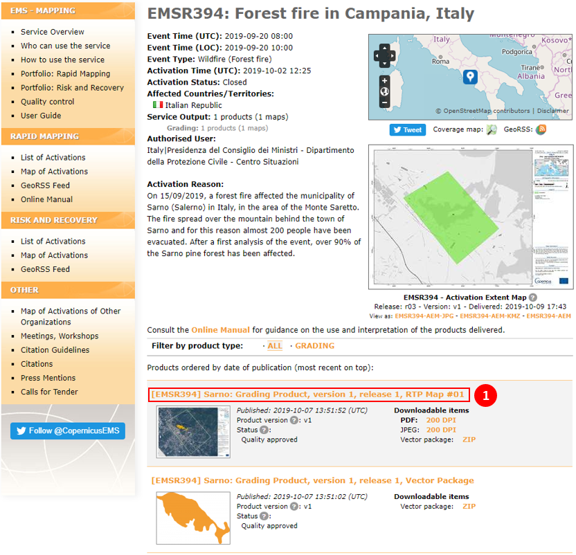
Inside the product page you will fing the preview for the delivered maps and vector datasets for the AOI for the activation. Here, download the vector package of the datasets delivered by the rapid mapping activities. Click on ZIP (1). In the following page, check the disclaimer box on the data use and proceed to Download file (2).
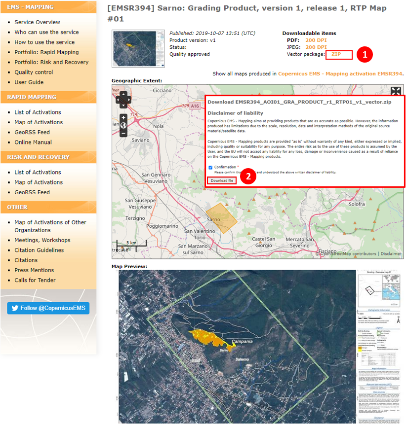
Fig. 4.2.2.6 –Copernicus EMS Rapid Mapping, Delineation product, Forest Fire in Campania, Italy. Vector Package Download (Gradiing EMSR394)
- Data Download - EOBrowser
Now that we have identified the AOI for the emergency, it is possible to follow the workflow as seen in Fig. 4.2.2.3.
Proceed to access the EOBrowser and Login with you user credentials.
Warning
This part of the practice implies that you have followed the lectures on “Sentinel Hub EO Browser” and that you are a registered “Sentinel-hub” user.
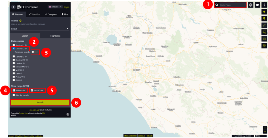
Fig. 4.2.2.7 –EOBrowser viewer. CEMS Rapid Mapping activation EMRS396 WildFire Event AOI.
Once that you have accessed the Sentinel-Hub your credentials you will have access not only to visualizing the catalogue in the browser, but also to the possibility of downloading the datasets. Now, we can define the querying parameters for our datasets of interest for the pre- and post-event of the fire (see Fig. 4.2.2.7):
Use the search bar located at the top-right of you screen and search for
Sarno, SA, Italia(1). Alternatively, you can move within the map canvas if you are familiar with the location, or you can upload a KML or GEOJSON file with the area of interest to identify the AOI.Data Source:
Sentinel-2(2)Advanced Search→L2A (atmospherically corrected)(3)
Time range:
- Start Date:`` 2020-09-01`` (4)
- End Date:
2020-09-30(5)
After successfully defining the query parameters, click on the Search button (6).
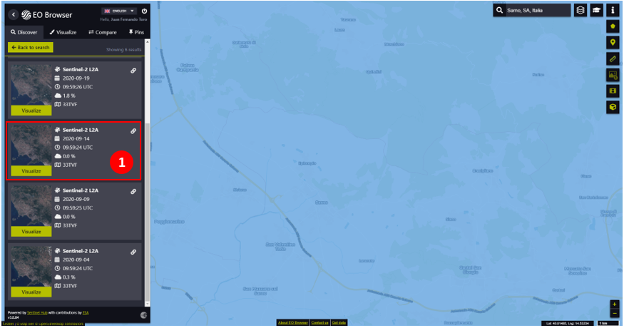
Fig. 4.2.2.8 –EOBrowser viewer. Available imagery fulfilling the parameters. EMSR394
Then, you will find the different imagery available for the current map view, which are intersecting or enclosing it. Here, from the list of available imagery matching the query parameters select the one for 2020-09-04 by clicking on visualize (1) as seen in Fig. 4.2.2.8 for the pre-event imagery.
At this point, the true colors imagery must be visible in the EO browser map viewer. In Fig. 4.2.2.9, click on the Download Image icon (1). A pop-up window will provide the options to define which products are of our interest and the type of file of the downloaded datasets. For the exercise, we will make use of the Near Infrared (NIR) and Shortwave Infrared (SWIR) Bands (i.e., B08A and B12, correspondingly). Select the Analytical tab (2) and complete the download form as follows:
Image format:
TIFF (32-bit float)(3)Image resolution:
HIGH(4)Coordinate system:
WGS 84 (EPSG:4236) (5)Layers: (6)
- Visualized:
True Color- Raw:
B08A,B12
Then, proceed to download the imagery by clicking on the Download button (7).
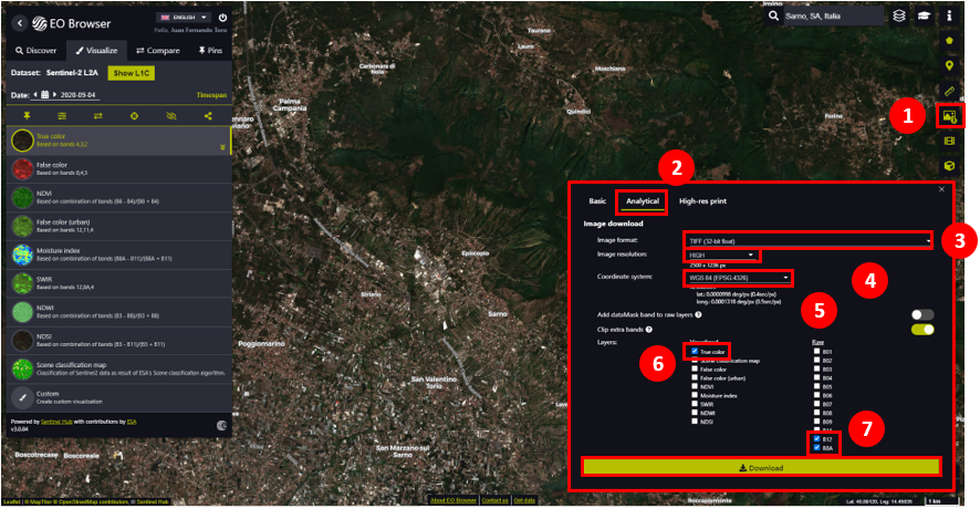
Fig. 4.2.2.9 –EOBrowser viewer. Wildfire event area of interest data download.
Note
This procedure requires that the map view completely encloses the AOI. The map extent will define the extent of the imagery retrieved from EOBrowser.
Warning
Do not toggle on the map canvas until having downloaded the datasets for pre- and post-event. In this case, the imagery retrieved depend on the map view.
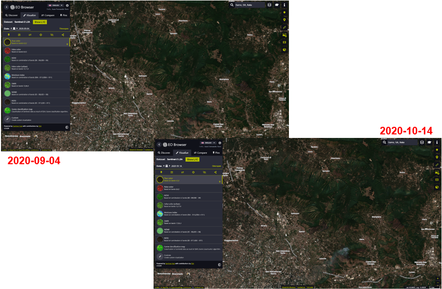
Fig. 4.2.2.10 –EOBrowser viewer. Flood event pre- (2020-09-04) and post-event (2020-10-14) view.
Now, for the post-event imagery in EOBrower, go back to the Discovery tab and select the imagery for 2020-09-14 by clicking in visualize. Repeat the procedure as presented in Fig. 4.2.2.9 to download the post-event images.
Note
Each of the pre- and post-event imagery are downloaded with a default naming that is “EO_Browser_images”. For the exercise, we will add to the files names “pre” and “post” depending on the date with respect to the event. The location of these files will be under the path .\Copernicus_EMS_Exercise\study cases\EMSR394 - Wildfire Scenario\EOBrowser-Scihub.
2020-09-04products are renamed as“EO_Browser_images_pre”2020-09-14products are renamed as“EO_Browser_images_post”
- GHSL-POP
In this part, you will download the population datasets which will support the assessment of the exposure of the inhabitants of the AOI with respect to the fire event.
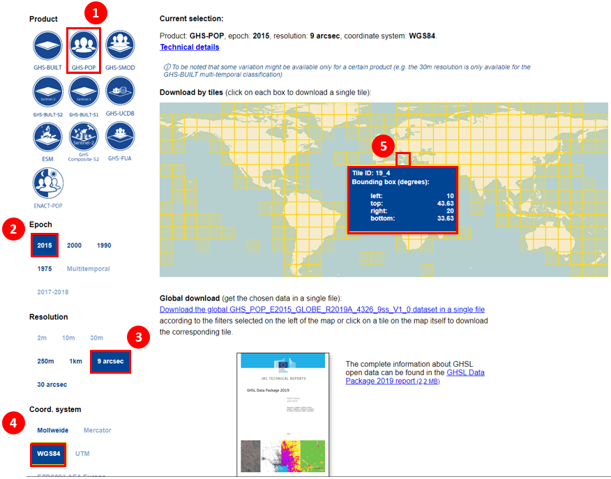
Fig. 4.2.2.11 –GHSL-POP 2015 dataset. Tile 19_4 data download. https://ghsl.jrc.ec.europa.eu/ghs_pop2019.php
The GHS-POP product of interest corresponds to the tile 19_4. Access the GHSL site. Select the parameters as detailed in Fig. 4.2.2.12:
- Product:
GHS-POPlayer (1)- Epoch:
2015(2)- Resolution:
9_arcsec(3)- Coord. system:
WGS84(4)
Once defined the parameters for the tiles layer, click on the tile 19_4 (5) on the map viewer. The downloaded file will be named as GHS_POP_E2015_GLOBE_R2019A_4326_9ss_V1_0_19_4. Proceed to move the file into the dedicated folder of the activation for the GHSL located in .\Chapter 4\Copernicus_EMS_Exercise\study cases\EMSR394 - Wildfire Scenario\GHSL.
Assessment of the impact of the fire
Warning
The upcoming steps require to have followed:
- Sections 1.4. - 1.9. in chapter 1. Data visualization with QGIS.
- Section 2.3. Extending QGIS functionalitites
- Section 2.5.5. Clip raster with a mask
- Section 3.4.1.8. Semi-Automatic classification Plugin Install.
Important
In this case, we have retrieved the imagery which has already been atmospherically corrected. For this reason, it is not necessary to apply any additional preprocessing.
Now, we can move to our desktop GIS to perform the damage assessment by overlaying the different datasets retrived until this point. In addition, the bands retrieved from the EOBrowser for the pre- and post-event will allow to model the damages on the vegetation due to the wildfire.
Add the imagery for pre- and post-event for Bands 8A and 12 (inside the layer group for the fire mapping activation). If the layers are not assigned into the corresponding group of layer drag and drop them into the correct one (see Fig. 4.2.2.12).
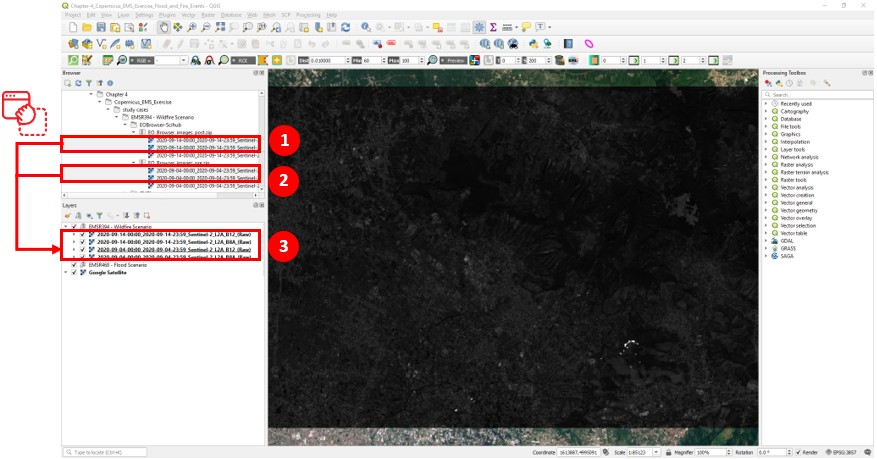
Fig. 4.2.2.12 – EMSR394 Fire Event in Campania Region. Pre- and post event imagery.
Let us recall that to compute the Normalized Burn Ratio (NBR), we must make use of Sentinel-2 NIR and SWIR bands as follows:
Note
In this case bands 8A (NIR) and 12 (SWIR) have been used to estimate the NBR. Recall from section 3.1.3.2. Multispectral Sentinel Satellites the applications of the spectral bands for Sentinel-2.
Warning
It is recommended to have done the 3.4. Hands-on exercises and that you have installed the “Semi-Automatic Classification” (SCP) plugin.
Here, we can make use of the SCP plugin. Go to SCP (1)→ Band Calc(2). There should be a window as presented in Fig. 4.2.2.13.
Note
In case that the bands list does not match with the layers that you are currently using refresh the window (3) (Fig. 4.2.2.13).
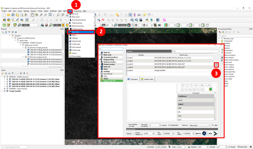
Fig. 4.2.2.13 –EMSR394 Fire Event in Campania Region. SCP raster calculator.
The band calculator, as the raster calculator, allows to execute operation in between multiple raster. Here, we are calculating the NBR for the pre- and post- event. The two estimates make possible to model the possible effects of the fire in the vegetation coverage. The changes in the vegetation coverage due to a fire event can be described through the NBR as follows:
In Fig. 4.2.2.14 the band calculator window is displayed. Here you can select the raster layers (1) and operations (2) to be executed within layers.
Compute the NBR for both pre- and post-event imagery using the following expressions:
- Pre-event NBR
(
"2020-09-04-00:00_2020-09-04-23:59_Sentinel-2_L2A_B8A_(Raw)"-"2020-09-04-00:00_2020-09-04-23:59_Sentinel-2_L2A_B12_(Raw)")/ ("2020-09-04-00:00_2020-09-04-23:59_Sentinel-2_L2A_B8A_(Raw)"+"2020-09-04-00:00_2020-09-04-23:59_Sentinel-2_L2A_B12_(Raw)")
- Post-event NBR
(
"2020-09-14-00:00_2020-09-14-23:59_Sentinel-2_L2A_B8A_(Raw)"-"2020-09-14-00:00_2020-09-14-23:59_Sentinel-2_L2A_B12_(Raw)")/ ("2020-09-14-00:00_2020-09-14-23:59_Sentinel-2_L2A_B8A_(Raw)"+"2020-09-14-00:00_2020-09-14-23:59_Sentinel-2_L2A_B12_(Raw)")
Fig. 4.2.2.14 shows the example for the computation of the NBR for the pre-event. Replicate the previous steps to obtain the same layer for the post-event.
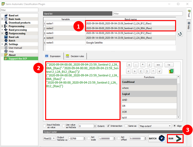
Fig. 4.2.2.14 –EMSR394 Fire Event in Campania Region. Example NBR computation (pre-event).
To build the expression displayed Fig. 4.2.2.14, you can refer to the layers by typing them in between quotation mark (“”), or by double-clicking on the layers in (1), the latter is the preferred solution, because it helps preventing mistyping. Replicate the expression as presented in (2). Then, click on Run (3). As the process is completely executed you will be prompted to input a path and name to the result of the expression. We will store the resulting dataset in the location and filename as follows:
- Path:
.\Copernicus_EMS_Exercise\study cases\EMSR394 - Wildfire Scenario\EOBrowser-Scihub- Filename:
pre-event_NBR
Repeat the previous procedure to obtain the NBR for the post-event. Use the following location and filename:
- Path:
.\Copernicus_EMS_Exercise\study cases\EMSR394 - Wildfire Scenario\EOBrowser-Scihub- Filename:
post-event_NBR
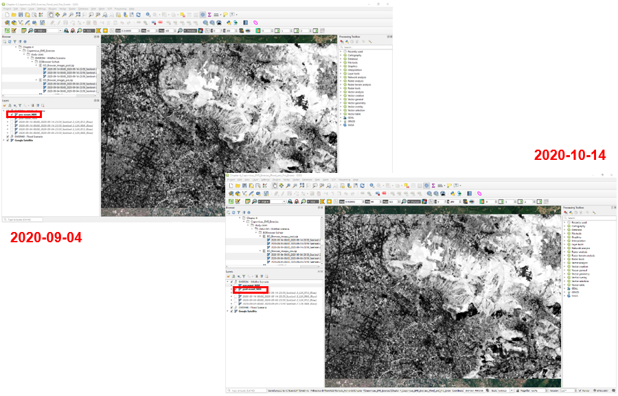
Fig. 4.2.2.15 –EMSR394 Fire Event in Campania Region. Pre- and post event imagery.
With the two NBR estimates, before and after the event, it is possible to map the burnt area. Open the “Semi-Automatic Classification” plugin raster calculator, on the menu bar select SCP → Band Calc to arrive to the window shown in Fig. 4.2.2.16. To highlight the burnt areas, write the expression:
"pre-event_NBR"-"post-event_NBR"
Make sure to refresh the bands list if the expected layers are not available as shown in (1). Write the expression in box (2) and proceed to Run (3) function.
Following the same procedure as for the NBR, we will save the file under the path:
- Path:
.\Copernicus_EMS_Exercise\study cases\EMSR394 - Wildfire Scenario\EOBrowser-Scihub- Filename:
event_dNBR
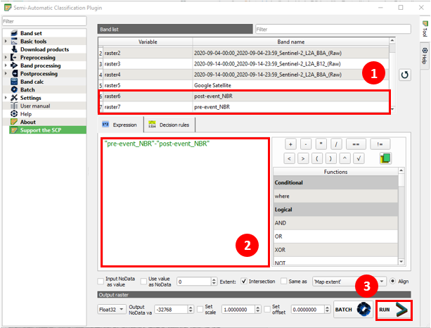
Fig. 4.2.2.16 –EMSR394 Fire Event in Campania Region. dNBR computation.
Notice that the layer has been added to your project. Make sure to place the NBR layers inside the “Wildfire Scenario”.
Warning
In general, the methodology would require applying a cloud mask to avoid that these elements are misclassified as fire. However, given that the imagery is cloud free for the AOI this step has been omitted.
Now we are going to limit the analysis area according to the AOI for the Copernicus EMS Rapid Mapping assessment. To add the shapefile you can either, find it on the browser panel on the upper-left part of the QGIS interface and doble-click on the layer, or retrieve it on the menu toolbar Layer → Add Layer → Add Vector Layer. In both cases, the layer can be found on the path:
- Path:
\Copernicus_EMS_Exercise\study cases\EMSR394 - Wildfire Scenario\Grading Products- Filename:
EMSR394_AOI01_GRA_PRODUCT_areaOfInterestA_r1_v1.json
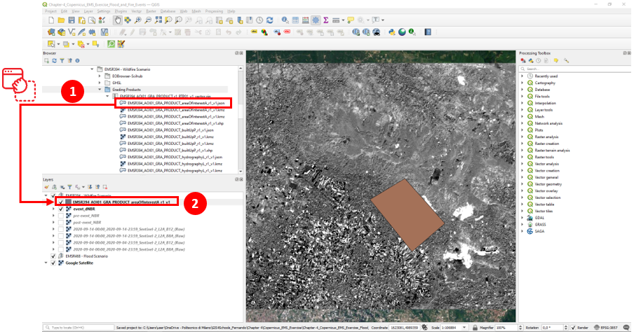
Fig. 4.2.2.17 –EMSR394 activation - Fire event AOI.
After adding the AOI shapefile, it should be available in the current grouped layer as displayed in Fig. 4.2.2.17. The AOI layer defines the extent for cropping the dNBR layer.
Next, we will provide to our representation some information concerning the porpulation living in the vicinity of the AOI. For this purpose, we will make use of the GHS-POP layers downloaded previously in the exercise. Add the GHS-POP tile to the working layer group. The file can be found here:
- Path:
.\Copernicus_EMS_Exercise\study cases\EMSR394 - Wildfire Scenario\GHSL\GHS_POP_E2015_GLOBE_R2019A_4326_9ss_V1_0_19_4.zip- Filename:
GHS_POP_E2015_GLOBE_R2019A_4326_9ss_V1_0_19_4.tif
Then, we will extract the information of the population layer within the AOI. For clipping the GHSL population layer we will make use of the “Semi-Automatic Classification Plugin”. On the toolbar menu select SCP → Preprocessing → Clip multiple rasters, later you will find again the SCP window (see Fig. 4.2.2.18).
The plugin enables the possibility to clip multiple raster bands at once by selecting them from the list of available layers (see Fig. 4.2.2.18). On the Band set tab (1) select the event_dNBR layer and add the layer into the list of layers to be clipped (either by double-clicking on the layer or selecting the layer and clickin on the + button (3)). Proceed to the tab Clip multiple rasters (4). The raster of the burn severity that is the band 1. You can also set a value for the NoData values but here we will leave the default value. Define the output name prefix as clip (here, the output for the clipped layer will have the name clip_event_dNBR). Now, enable the Use vector for clipping (5) option and select the vector layer defining the extent to crop the raster imagery (EMSR394_AOI01_GRA_PRODUCT_areaOfInterestA_r1_v1) (6). Finally, you can execute the command to obtain the clipped image. When the proccess finishes save the resulting file in the folder Copernicus_EMS_Exercise\study cases\EMSR394 - Wildfire Scenario\EOBrowser-Scihub.
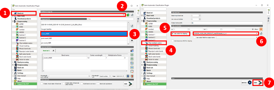
Fig. 4.2.2.18 –EMSR394 activation - SPC multiraster clip.
Search the resulting layer for the burnt areas (clip_event_dNBR) (1) and add it into the group of layers for the fire event (2) (see Fig. 4.2.2.19).
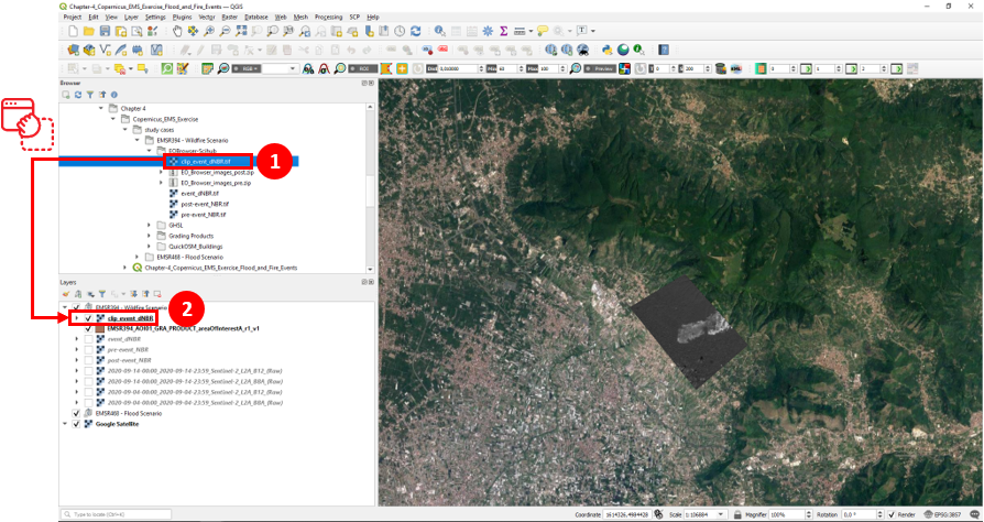
Fig. 4.2.2.19 –EMSR394 activation - Clipped burn severity layer.
Next, a symbology is provided to the dNBR Layer. To provide a better understanding of the layer through its view, we will proceed to define a symbology. According to the USGS standard for burn severity mapping the following set of ranges shown in Table 4.2.2.1 should be considered. Access the symbology options for the layer by right-clicking on the layer name clip_event_dNBR → Properties... → Symbology tab. Now, we are in the symbology properties window for the layer (see top box in Fig. 4.2.2.20). First, on the Render type select the Singleband pseudocolor. Then, open the drop-down menu for the color ramp and click on the Create New Color Ramp... option (1). In the new window, select the Color Presets options and click on ok (2). At this point, we will define the colors composing custom the color ramp. Modify the exsting symbol by double clicking on it (3). Now, you can define a color to the symbol through the HEX code (4) (use the HEX coding in Table 4.2.2.1) and then confirm the color choice OK (5). Change the label of the color providing an appropriate description of the color (6). Continue to define the color ramp by adding new symbols (7) and editing them until including all the categories to represent the burn severity.
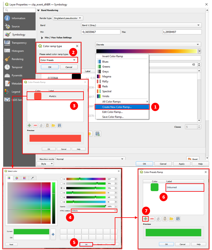
Fig. 4.2.2.20 –EMSR394 activation - Burn severity symbology.
Fig. 4.2.2.21 presents the complete customized color ramp. Once finished, click on OK to confirm the submission of the color ramp, Classify the layer according to the symbology and proceed to apply the changes to the layer by clicking on OK.
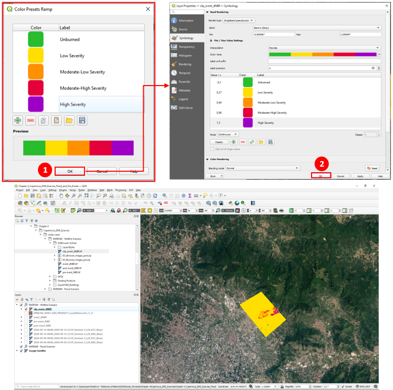
Fig. 4.2.2.21 –EMSR394 activation - Burn severity classification.
Alternatively, you can modify the layer symbology through a text file. This can be achieved in the symbology properties by selecting the folder icon next to the classify button. You may find the styling text file under the path:
- Path:
.\Copernicus_EMS_Exercise\study cases\EMSR394 - Wildfire Scenario\EOBrowser-Scihub\LayersStyles- Filename:
dNBR_customized.txt
The following step requires to include the GHS-POP raster in the group of layers. After this, clip the layer using the Clip raster by mask layer (see Fig. 4.2.2.22). If the processing toolbox is not available in the right hand of your QGIS user interface, select from the menu bar Processing (1) → Toolbox (2). In the Processing Toolbox pane, type in the search bar clip (3) and select the Clip raster by mask layer function (4). Then, define the following parameters to crop the raster:
- Input layer:
GHS_POP_E2015_GLOBE_R2019A_4326_9ss_V1_0_19_4 [EPSG:4326](5)- Mask Layer:
EMSR394_AOI01_GRA_PRODUCT_areaOfInterestA_r1_v1 [EPSG:4326](6)Provide the path and naming for the output file:
- Clipped (mask):
.\Copernicus_EMS_Exercise\study cases\EMSR394 - Wildfire Scenario\GHSL\GHS_POP_E2015_GLOBE_R2019A_4326_CLIP.tif(7)- Activate the option
Open output file after running algorithm
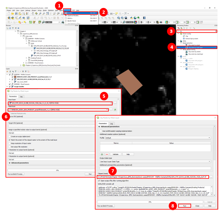
Fig. 4.2.2.22 –EMSR394 activation - add and clip the GHS-POP 2015 layer tile 19_4.
With the clipped AOI, now it is convenient to define a symbology to the layers to highlight the presence of the population. Open the clipped GHSL-POP layer symbology properties (see Fig. 4.2.2.23). First, select the Tranparency (3) tab and define a transparency percentage (4) to the layer. Then, move to the Symbology tab (5), select the Discrete (6) as Interpolation and replace the color ramp highlighting concentration, smooth to strong colors, in this case of people (7). Choose the categories mode as Equal interval (9) for 5 different classes (10). Use Classify (11) button and then click on OK (12).
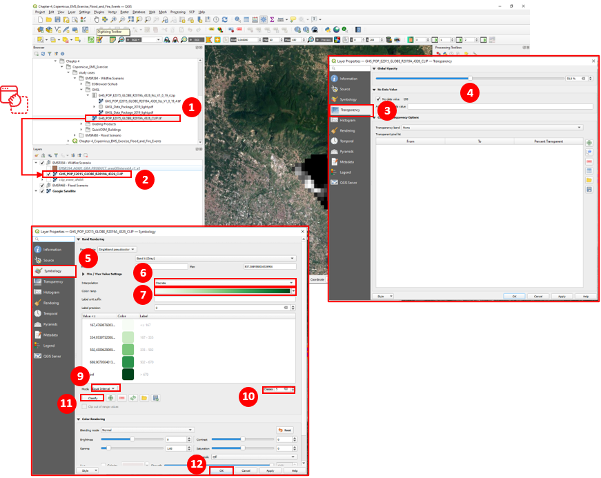
Fig. 4.2.2.23 –EMSR394 activation - Clipped GHS-POP tile 19_4 symbology.
At this point we can import the last dataset to be used for this project that is the presence of built environment within the AOI. For this purpose, we will extract the features for the buildings in the AOI guided by the steps in Fig. 4.2.2.24. On the menu bar select Vector (1)**→ ``QuickOSM`` **(2)**→ ``QuickOSM…`` **(3). As the querying parameters:
- key:
building- value:
yes
Open the advanced options for the plugin (7) and define the path to the folder to store the retrieved vector datasets (8).
- Path:
\Copernicus_EMS_Exercise\study cases\EMSR394 - Wildfire Scenario\QuickOSM_Buildings
Finally, execute the plugin and click on OK (9)
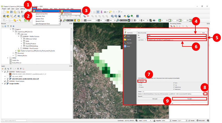
Fig. 4.2.2.24 –EMSR394 activation - Query building features from OSM.
If at completition of the execution of the QuickOSM plugin the layers were not added to the map, you can retrieve and add them through the browser panel as done previously for other layers (see Fig. 4.2.2.25).
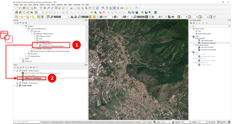
Fig. 4.2.2.25 –EMSR394 activation - Query building features from OSM.
Create a new layout to present the results from the analysys.
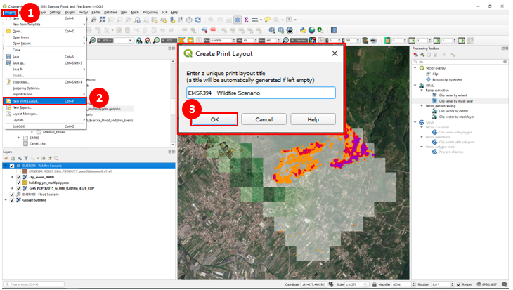
Fig. 4.2.2.26 –EMSR394 activation - Compose a new layout with the burn severity estimates.
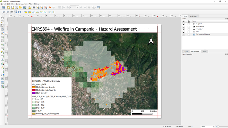
Fig. 4.2.2.27 –EMSR394 activation - Burn severity compose layout.
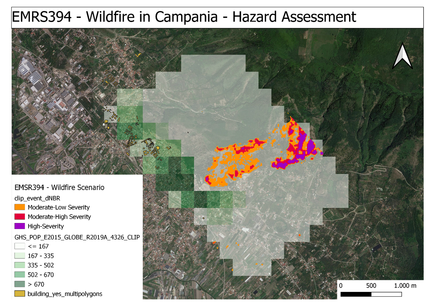
Fig. 4.2.2.28 –EMSR394 activation - Burn severity map.
4.2.3. Other Useful Resources
- Global Human Settlement Layer
The Global Human Settlement Layer (GHSL) project produces timely geospatial information of human presence on the planet. Through the used of spatial data mining technologies, the project harvests information with evidence-based analytics and knowledge. The information is exposed as built-up maps, population density maps and settlement maps. The GHSL profits from the use of heterogeneous data such as satellite imagery, census data, and volunteered geographic information.
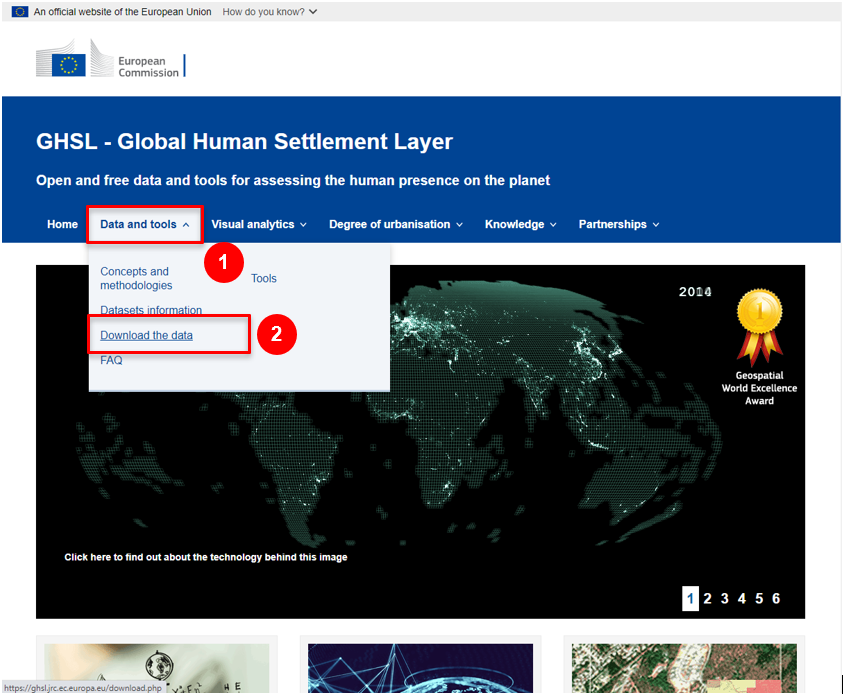
Fig. 4.2.3.1 –Global Human Settlement Layer website, https://ghsl.jrc.ec.europa.eu/
- Global Human Settlement Layer (GHSL) - Population
The Global Human Settlement Layer Population layer (GHSL-POP ) [2] is a spatial raster dataset depicting the distribution and density of the population expressed in number of people by cell. The production of this imagery is possible through the disaggregation of census or administrative spatial data into cells. Values are expressed as decimals (Float) and represent the absolute number of inhabitants of the cell. The residential population targets the years 1975, 1990, 2000 and 2015. The GHSL-POP datasets can be described by:
- Product name: GHS_POP_MT_GLOBE_R2019A
- Coordinate System: World Mollweide (EPSG:54009), WGS (EPSG:4326)
- Resolution available: 250m, 1km, 9 arcsec, 30 arcsec
The naming convention for the GHSL-POP datasets is defined as “{Product Name}_{Coordinate System}_{Resolution}_{Version}” (e.g. GHS_POP_E2015_GLOBE_R2019A_4326_9SS_V1_0, that is the version 1 of GHSL-POP dataset for 2015 referred to WGS84 with a resolution of 9 arcsec).
Note
NoData cells are assigned -200 as value.
After following the steps as presented in Fig. 4.2.3.1, you will find a web viewer visualizing the tiles for the GHSL-POP products. At this point you can click on the tiles of enclosing your area of interest and execute the download of the raster dataset.
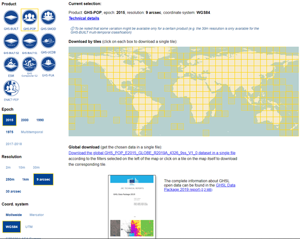
Fig. 4.2.3.2 –Global Human Settlement Layer Population Tiles Web Viewer, https://ghsl.jrc.ec.europa.eu/ghs_pop2019.php
| [2] | Schiavina, Marcello; Freire, Sergio; MacManus, Kytt (2019): GHS population grid multitemporal (1975, 1990, 2000, 2015) R2019A. European Commission, Joint Research Centre (JRC) DOI: 10.2905/42E8BE89-54FF-464E-BE7B-BF9E64DA5218 PID: http://data.europa.eu/89h/0c6b9751-a71f-4062-830b-43c9f432370f. |