2.6. Graphical modeler
Visual programming is a programming language that uses illustrations instead of text (code). In this way, the user can define a process in a form that is more understandable for humans, while writing scripts he must adapt his thinking to the computer way. As for scripting, the final outputs are algorithms including a series of simpler operations, usually associated with software commands.
The Graphical modeler is the visual programming interface of QGIS and allows to create models, even very complex ones, that chain a series of operations on some inputs in order to produce some outputs. This is particularly useful because most of the analysis usually performed in a GIS environment involves many different operations in series. Creating a model that resumes all these operations allows to run the whole analysis as a single process, saving time and even reducing the risk of distraction errors. The Graphical modeler algorithms can be seen as a visual representation of workflows.
In this lecture, we will create a model reproducing some of the operations performed in the Vector Processing part. In this way, it will be possible to compare the two alternative ways of proceeding focusing on the graphical modeler dynamics, spending only a few words on the description of the operations as we already met them. We are going to use the following vector files:
- Lakes.shp (polygons representing the main lakes of the area of interest);
- River_network.shp (lines representing the river network across the lakes basins);
- Municipalities_OSM.shp (polygons representing the boundaries of the municipalities).
To start, add the Vector layers (see Fig. 2.6.1, 1) to your project. Right click on one of the upper toolbars and flag the box of the Processing Toolbox Panel to visualize it on the right (2). From the search bar on the top of it (3) all the operations of QGIS and its plugins (including GRASS, GDAL and SAGA) can be found and used. This way of looking for a command is fast and allows us to find some operations that we don’t know exactly the name or the path. Nearly all the same operations are available also within the Graphical modeler. To open it, click on Processing (4) and then select the second option, Graphical modeler (5).
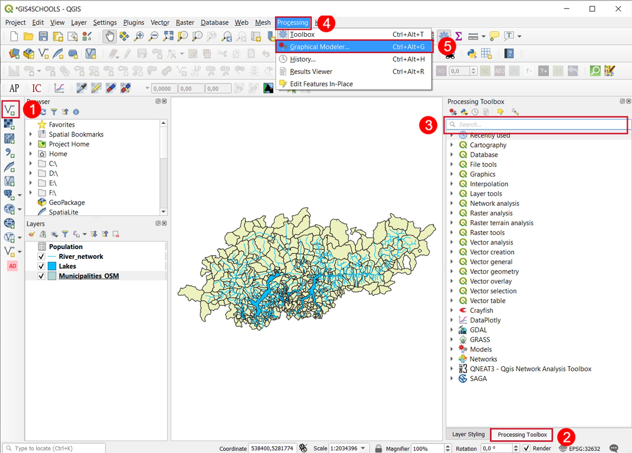
Fig. 2.6.1 – Add layers, display processing toolbox and launch the Graphical modeler
A new window called Model Designer will open (Fig. 2.6.2). Here, three main parts can be distinguished. First, an upper toolbar that will be better explained in Fig. 2.6.8, then a left column, and an empty white space that we’ll call canvas. The first section of the left column contains the Model Properties (Name 1, Model 2) that need to be set in order to save a model. The Algorithms section below works exactly as the Processing Toolbox Panel seen in Fig. 2.6.1 and will be used during the following steps of the exercise. The last part of the left column is dedicated to the Inputs. Inputs can be added to the canvas by double-clicking on them or by drag and drop. They work as empty boxes with some constraints that will be filled by a specific layer when we’ll run the model, once completed. In this case, we need to select three times the Vector Layer input (3) to host three different layers. The Vector Layer Parameter Definition window (4) opens and allows us to define the characteristics of the layers that will be acceptable in a specific box. The first one is intended to host the Municipalities_OSM layer. As Parameter name (5) we set Cities to remind that we are dealing with administrative boundaries but also to show that it doesn’t need to be labeled in the same way as the layer that will contain. As Geometry type (6) select Polygon from the drop-down menu. The Comments tab (7) allows to input a description to help future the users understanding the model and it’s included also in the operations windows. Select a Colour (8) with whom it will be displayed on the canvas and click OK (9). A yellow box named Cities (10) appears on the canvas and is ready to be connected with operations, together with a light blue box with the comments text (11). Repeat the same operation for Lakes (polygon) and Rivers, choosing line as geometry type. We can see the other two options included in this window (12). There’s the possibility to define if these parameters are Mandatory and/or Advanced. As the advanced parameters won’t immediately appear to the user when running the model, it’s better to flag this checkbox only for non-mandatory parameters. In this exercise, all the parameters will be mandatory and non-advanced. Clicking on OK also the Rivers box (13) appears on the canvas.
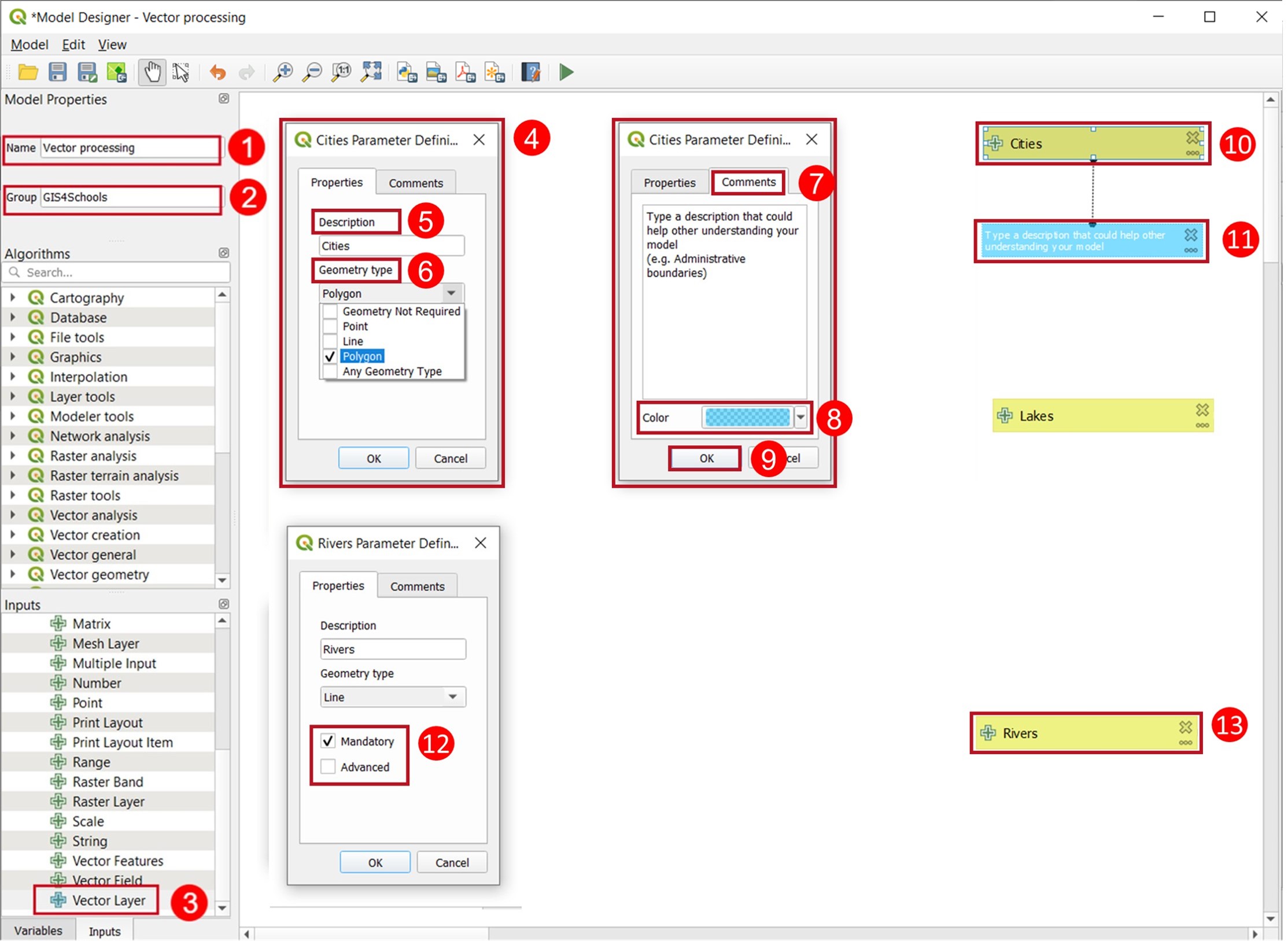
Fig. 2.6.2 – Graphical modeler window overview and input definition
Once defined the inputs, we can start adding the steps of our process (Fig. 2.6.3). Every step is an operation that can be found in the Algorithm section of the left column by typing in the search bar (1) its name. We now want to create a new field for the Cities input containing the area of each feature. Typing “field” in the Search box, a set of functions with the word field in their name appear, together with others dealing with fields. Among those, select Field calculator (2) and double click on it to open the homonym window (3). Here we need to define all the different parameters required for an operation, exactly like we do in the manual mode. In the Description field (4) we find by default the operation’s name but it can be modified. The Description is also how the operation is displayed on the canvas white box (15). For the inputs we have different options. Clicking on the icon (5) a drop-down menu appears (6). As Input layer (7) we select the option Model Input while for all the others we leave the default option (Value). In this way only the previously defined inputs (Cities, Lakes and Rivers) can be selected. Set Cities as Input layer, Area as Result field name (8), Float as Field type (9), 18 as Field length (10), and 2 as Field precision (11). In the Formula space (12) we type $area. An alternative to the embedded expression editor for more advanced users is the Function editor (13), that allows integrate python scripts. Click on OK (14) and a white box (15) appears on the canvas, with In (input) black dot connected to the Cities box through a wire.
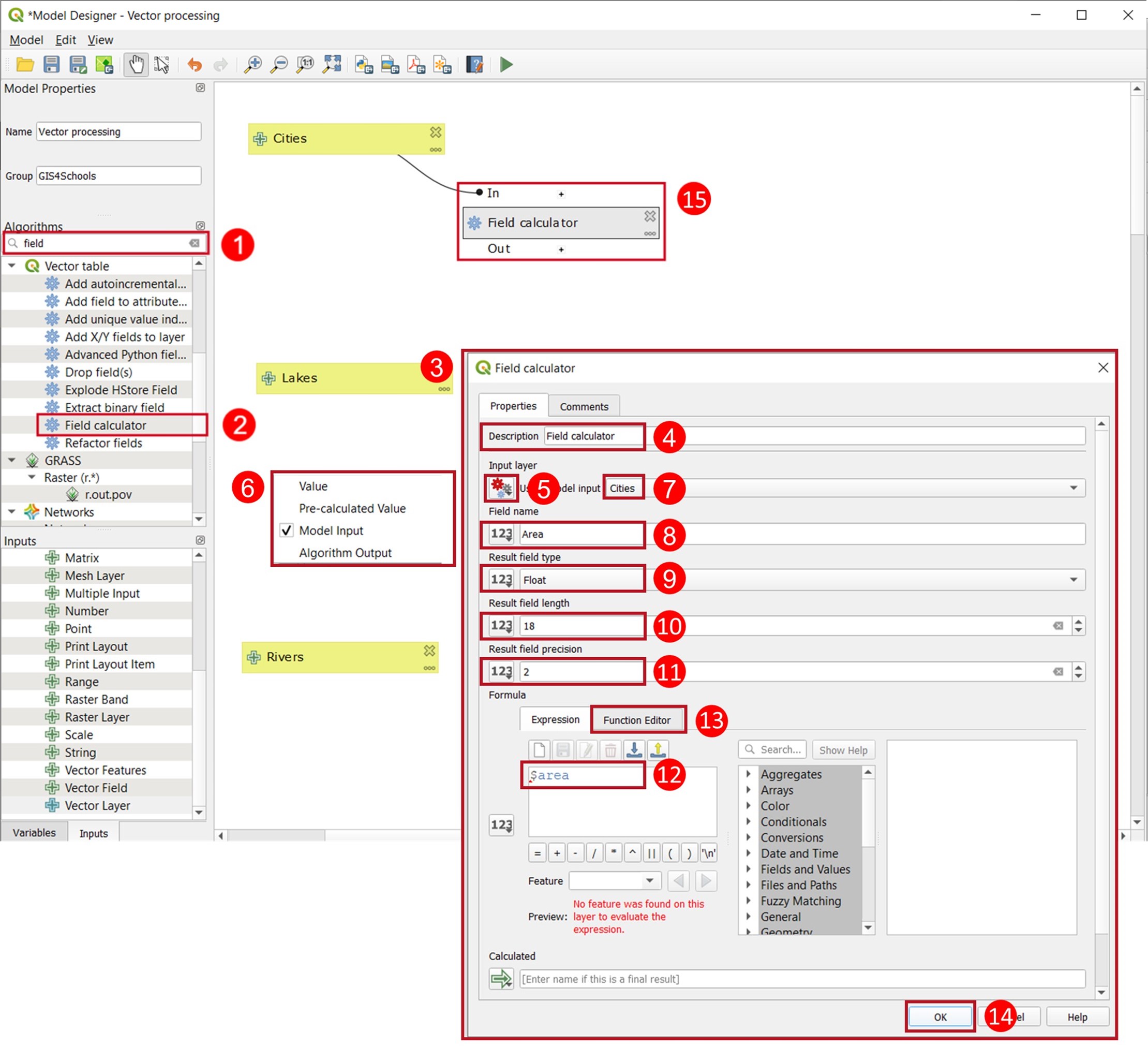
Fig. 2.6.3 – Algorithm search and Field Calculator, example of single input operation
In chapter 2.4 we first selected by location the Municipalities intersecting the Lakes layer and then exported them. Here (Fig. 2.6.4) we make it with a single operation called Extract by location (1). In the homonym window (2) we see that two inputs are required: the Municipalities and the Lakes layers. As we previously modified the Cities input adding one field, we can no more use the original input but rather refer to the result of the last operation performed. So, we Extract features from the “Calculated from the algorithm Field Calculator” (3), an algorithm output (to be selected among the input options), By comparing to the features from “Lakes” (4), leaving the intersection as the default geometric predicate. Click OK (5) and the corresponding white box appears on the canvas (6) with two wires entering the In dot.
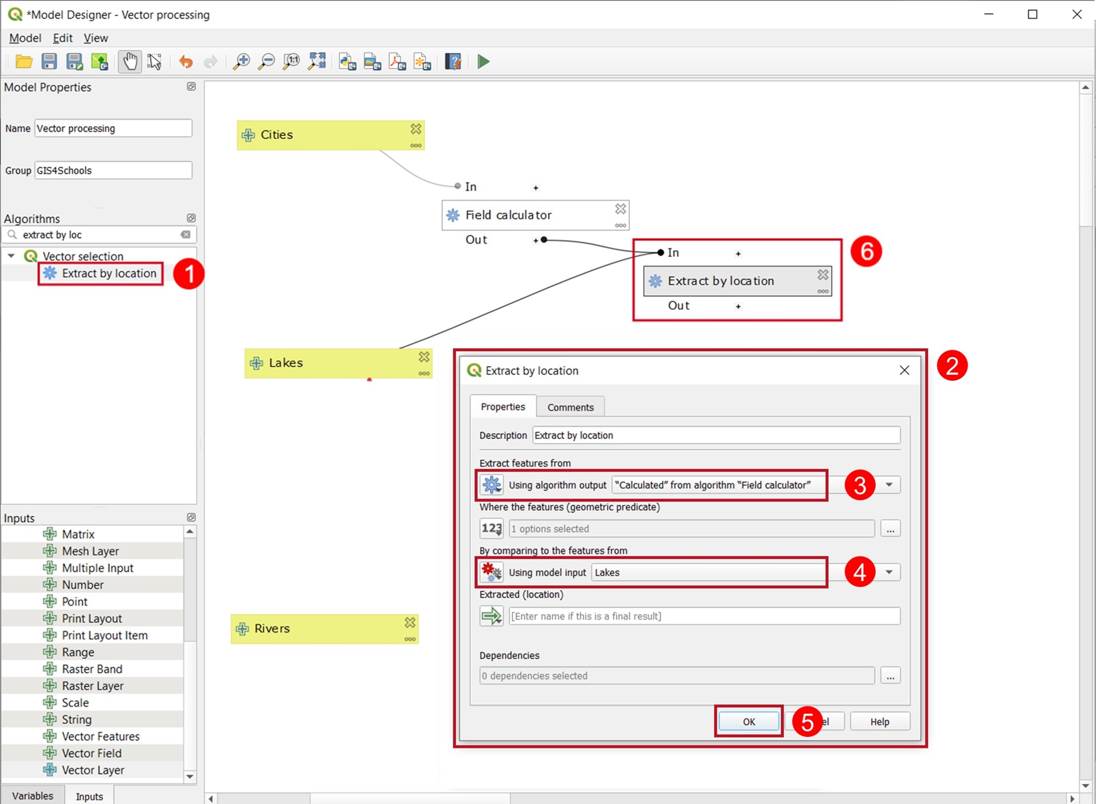
Fig. 2.6.4 – Extract by location, operation involving more than one input
Conclude the operations related to the Cities input with Dissolve (Fig. 2.6.5, 1) using the result of the last step, creating a vector layer corresponding to a Region of Interest around the Lakes. In the Dissolve window (2) select the “Extracted (location)” (3) from the drop down menu of the Input layer. As you can see the output of an operation is labeled using the past participle of the operation name (calculate/d, extract/ed) with some exceptions. To define the Dissolve field we need to know the layer that will be used as input for the Cities box. To avoid this, having more flexibility in the definition of the parameters, this field must be defined as model input, as done for the vector layers. This option will be shown later, at the moment manually set NOME_PRO (4) as Dissolve field. The last field (5) to be filled is the one controlling the creation of final output to QGIS and can be identified by the placeholder [Enter name if this is a final result]. This section has a different name from operation to operation often using the past participle of the operation verb. Even if here it is called Dissolved, we can refer to it as the Output field. The outputs generated will be temporary files and are visible on the canvas, together with the operation white box (6), as green boxes (7).
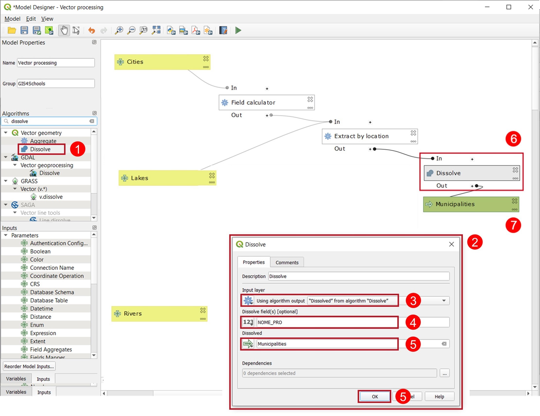
Fig. 2.6.5 – Dissolve and creation of outputs to QGIS
Proceed in the lower part of the canvas making an Intersection between Lakes and Rivers inputs without specifying additional parameters. Connect then the result of the Intersection, a set of river segments, to a Field Calculator to add a new field called Length (type: float; length: 12; precision: 2; Formula: $length). In the Description, add a 2 after Field Calculator to distinguish it from the one previously used.
Connect the last box to a new Field Calculator (Fig. 2.6.6, 1) that will divide the river segments in two categories according to their length. Call this new field 50km (2) and select Integer as Type (3) and 2 as Length (4). In the Formula field (5) type:
if("Length" > 50000, 50, 20)
The meaning of this expression is to assign a value of 50 to the river segments longer than 50000m (50km) and a value of 20 to those that are shorter. Click OK (6) to visualize the box on the canvas (7). Notice that the progressive numbers (manually set) beside Field Calculators have been highlighted to show their importance to distinguish the different homonym operations within a model. We can use the Formula field (5) to show different options with respect to the manual input. A demonstrative Expression dialog window (8) shows how the same expression could be written in order to give a growing level of control to the user when running the model. The first expression leaves no editing possibility as everything is predefined, but all its elements could be replaced by a model input. In the second one, e.g., the value of 50000 has been replaced by a Number parameter called threshold. In the third one, also the field “length” has been replaced with an homonym Vector Field parameter. The two can be distinguished by syntax and color in the expression. Fields are in orange and in quotes (“…”) while input parameters, no matter their type, are in light blue and preceded by a @ symbol. The last expression directly refers to an Expression parameter, allowing the user to write the whole expression from scratch at every model run. The elements in the expression space and the corresponding input boxes and windows have been underlined with the same color to help understanding the figure.
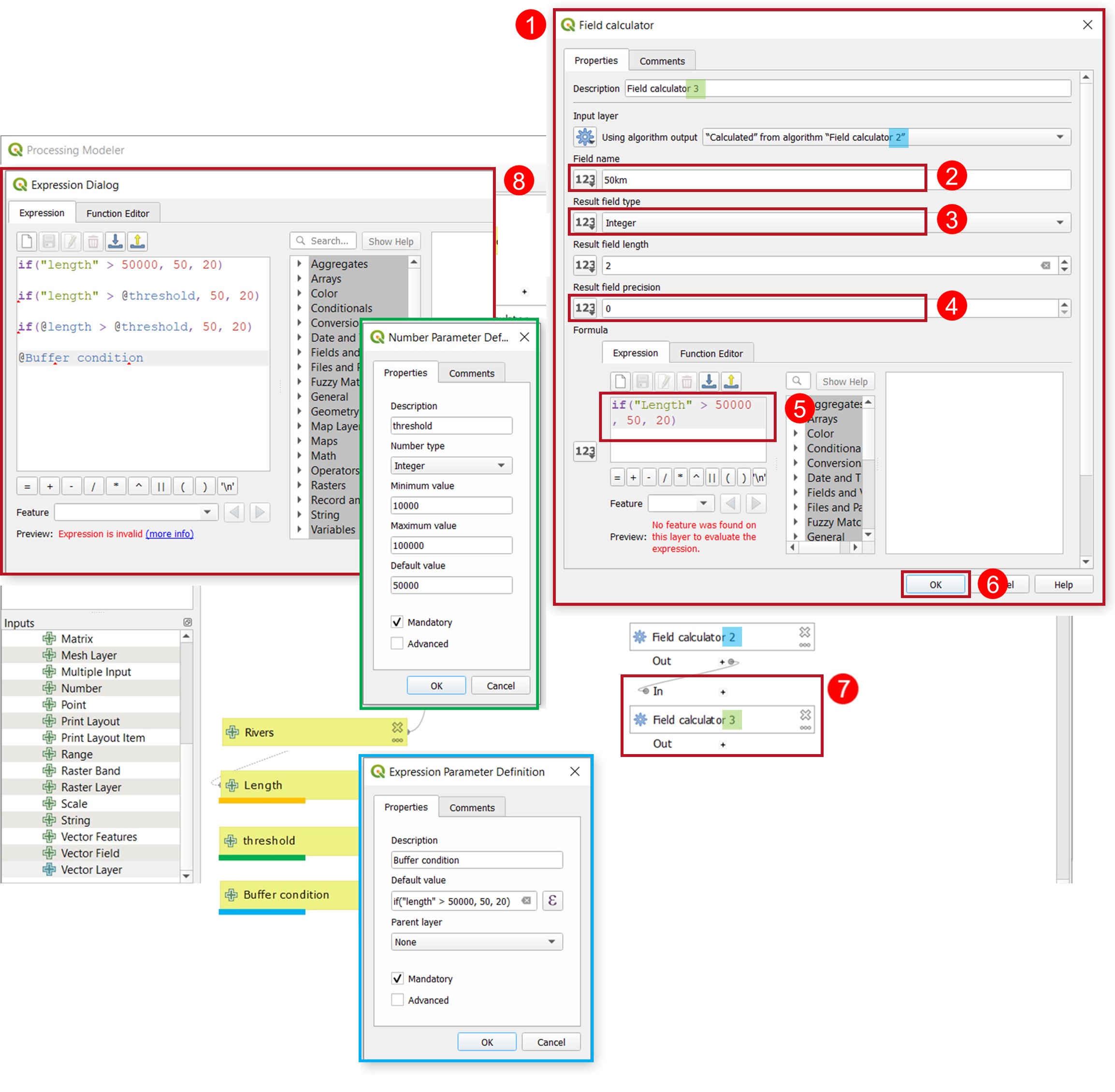
Fig. 2.6.6 – Field Calculator 3 and a focus on the different possibilities to input an expression
The last step of the model is the creation of a Variable distance buffer over the river segments according to the 50km field returning an output to QGIS called River_Buffer. Fig. 2.6.7 shows the final model completed and ready to be run.
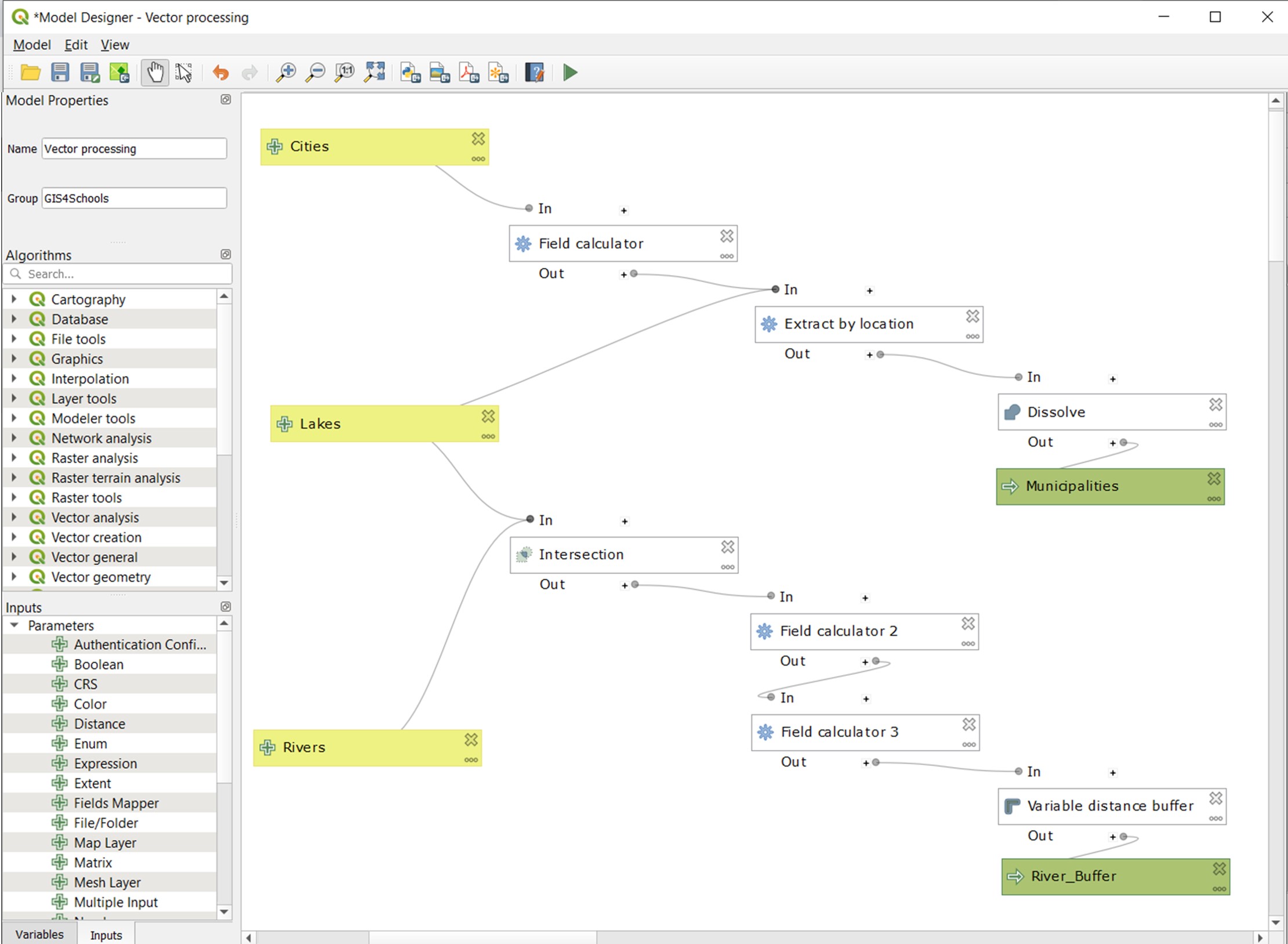
Fig. 2.6.7 – Completed model with inputs (yellow), operations (white) and outputs (green)
Now that the model is complete we can explore the functionalities contained in the upper Toolbar (Fig. 2.6.8). The first three icons are the classic Open, Save and Save as commands (1). Models have a .model3 extension and when saving them, it can be useful to save a copy both in the default path and in a more accessible folder. There is also the possibility to save the model within the current project (2). In this way, no .model3 file will be generated and the model will be accessible through the Processing toolbox panel in the Project models section to be executed or edited. Next two icons (3) allow to switch between the Pan Layout, used to move inside the canvas, and the Select/Move item, used to move and edit boxes. After that we find the classical Undo/Redo icons (4). A set of Zoom options (5) allow better navigation of the canvas. The icon Export as script algorithm (6) opens the Processing script editor (7) where the model is translated in a text-based python programming language. This could be helpful for beginners to improve their programming skills by comparing it with the visual model and also to make minor modifications directly inside the script. Edited scripts can be saved and run, opening the window shown in Fig. 2.6.9 by clicking on the same icon in the upper Toolbar (14). The visual representation of the model can be Exported in different formats (.jpg, .pdf, .svg, 8). There is the possibility of creating a model Help (9) by editing a predefined template, visible in the Help editor window (10). Here, we need to select an element to edit (11) in the bottom left list, type its content in the bottom right text space (12) to update the upper box (13) with information that might be useful to users to better understand the model. Finally, the Run model (14) icon allows it to be executed.
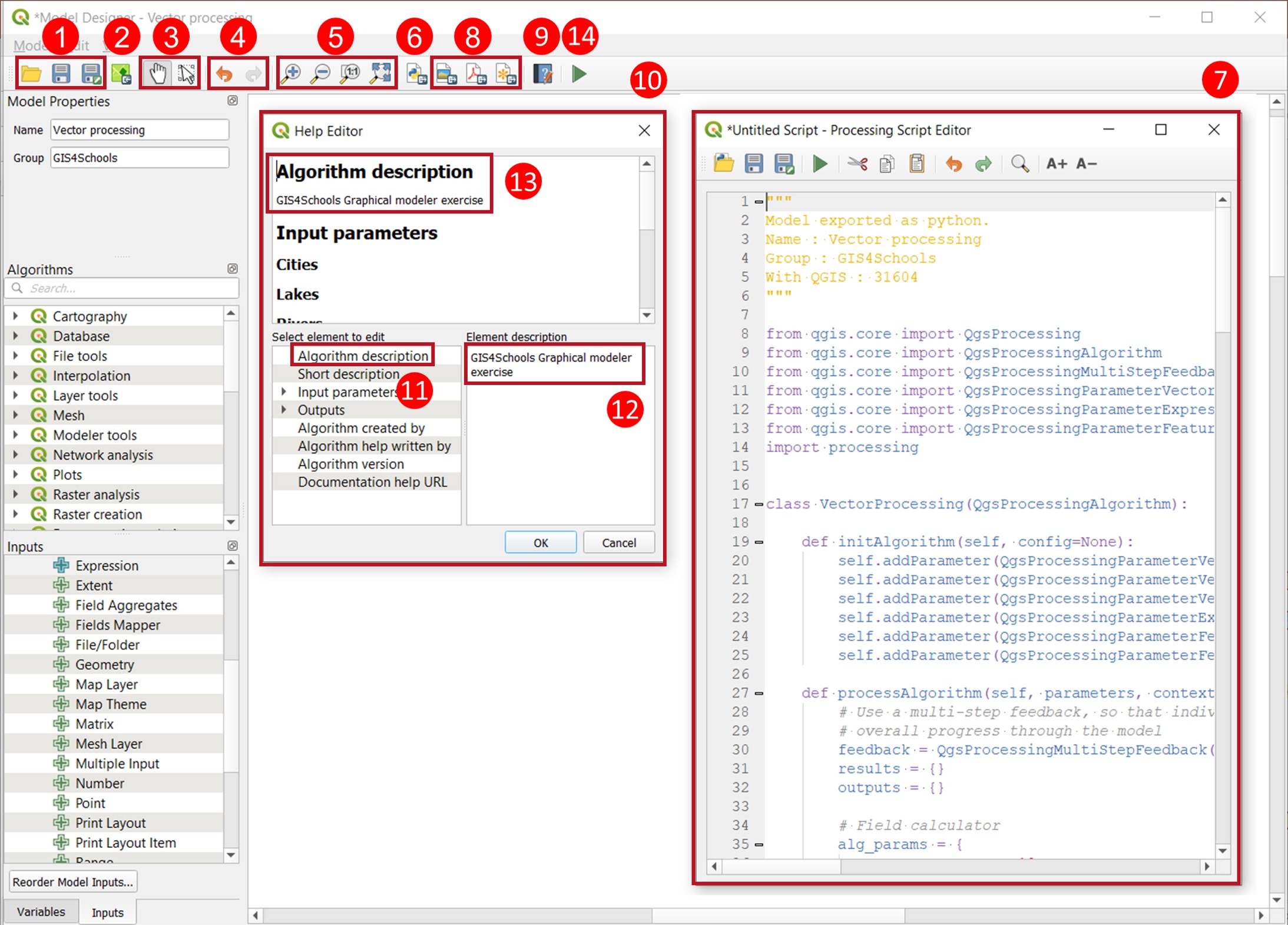
Fig. 2.6.8 – Graphical modeler toolbar with save, zoom, export and help options
A window named as our model and very similar to the classic operations windows opens and we are asked to select one layer for every input (Fig. 2.6.9). In the right column (1) the content of the Model Help is reported. Layers can be both selected among the ones loaded in the project, visible in the drop-down menu, or even from a file path (2). Set as input Municipalities_OSM for Cities (3), Lakes for Lakes (4), and River_network for Rivers (5) and click on Run (6). A window showing the progress of each model step, in the text, and of the overall model on the bottom blue bar will appear (7) and, when finished, the model outputs become be visible in QGIS both on the map and in the Layer Panel where two temporary layers (Municipalities and River_Buffer) appear. They can be exported to become stable layers saved in a file path.
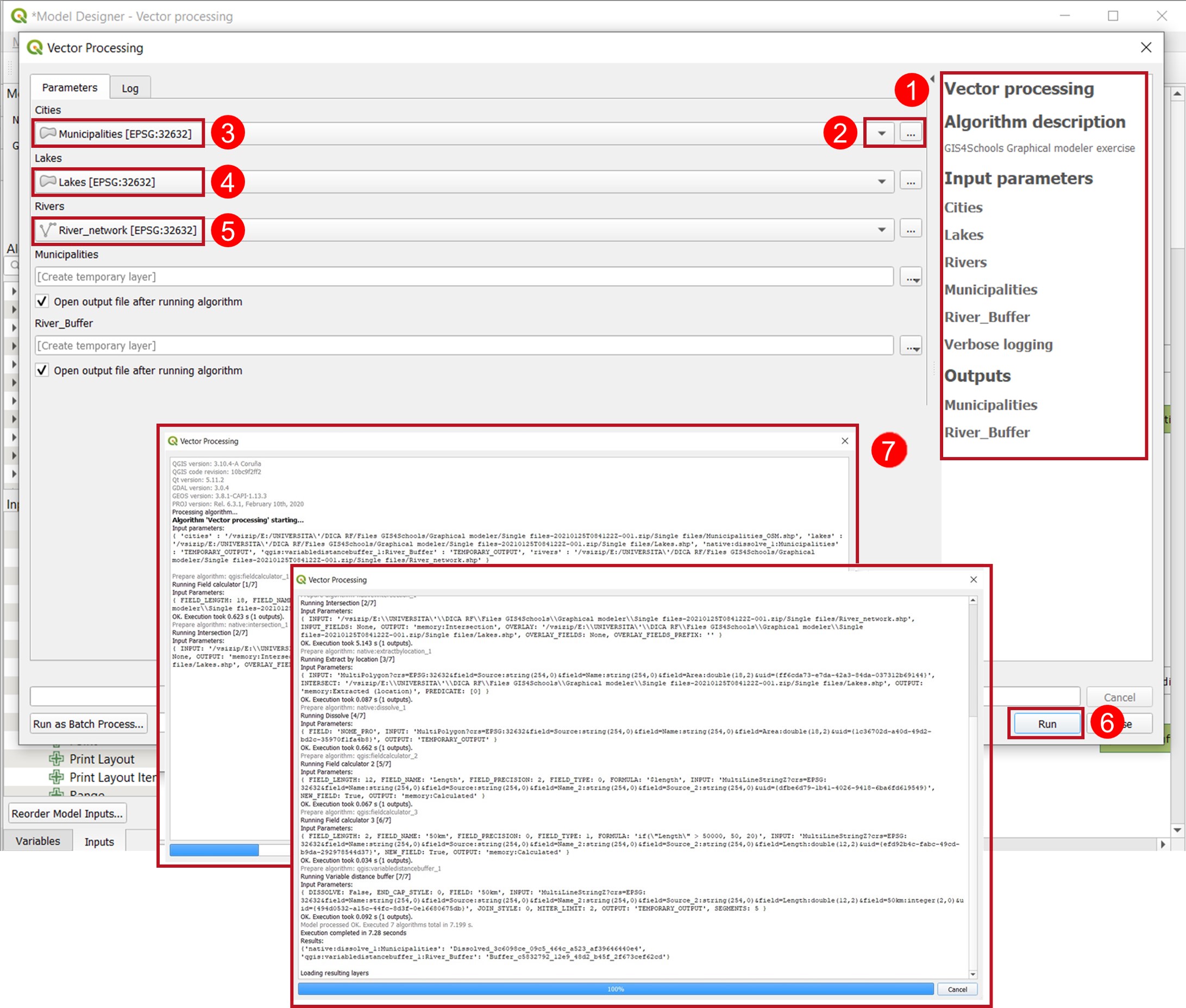
Fig. 2.6.9 – Run window for input definition and progress of the model
References: