1.3. GIS data modelling

Once the mathematical procedures to link data with their geographic locations are defined, it is critical to GIS to identify models that encode this information in a computer environment. These models, known as GIS data models (or geospatial data models), are a set of constructs and abstractions for describing and representing geographic entities in a digital system. Basically, GIS data models reshape these entities into discrete geographic objects (vector models) or continuous surfaces (raster models) and fit both numerical and/or textual attributes with coordinates into computer files. The structure of these models is independent of specific data items and, in most cases, of the particular GIS application that is used to manipulate them.

GIS data models are often interchangeable so that the same geographic entity or phenomenon may be represented by different models. As an example, topographic relief of mountains may be portrayed as a continuous surface or as a series of lines (discrete objects) representing contours of equal elevation. Conversions between models entail some costs both computationally and in data accuracy but GIS software provides functions to perform automatically such conversions.

The right data model to use strictly depends on the specific application. What is important to keep in mind is that there is no single data model that is best for all circumstances. Nowadays, GIS software is able to incorporate multiple data models and so can be applied to a wide range of different applications.

1.3.1. Raster data

Raster data models describe geographic entities as a matrix of pixels or grid cells. The entities of interest are represented by numeric values associated with each cell, and the coordinates of the cell center (or one of its corners) are encoded together with values in the raster data file (Fig. 1.3.1.1). The cell value can represent a wide variety of information. This includes categories as well as the magnitude of a measurable variable. As an example, categories could represent the land cover class or the soil type which is present at a cell location. Magnitudes might instead represent temperature, surface elevation above sea level but also the intensity of light radiation as seen by a digital camera. Cell values can contain either positive or negative integers or floating-point values. Integer values are suitable to represent categories while floating-point values best represent continuous geographic phenomena in which values change gradually over broad areas. Cells can also contain NoData values to represent the absence of data in those locations. Raster data can be encoded in many file formats. One of the most widely adopted raster data formats in GIS is the GeoTIFF.

Typically, raster cells are square and evenly spaced in the x and y directions. The spacing of cells is often referred to as spatial resolution. Spatial resolution is one of the major aspects to consider in working with raster data because it directly influences the accuracy in portraying geographic entities achieved by the raster data. The spatial resolution strongly influences (together with the extension of the mapped area) also the dimension in the computer memory of a raster data file. Specifically, the higher the spatial resolution (i.e. the smaller the cell) the better is the level of detail provided by the raster data while the data file dimension increases. However, mathematical operations on raster data are generally computationally faster than, for example, vector data. This is due to the regular matrix format of raster data that can be easily handled by GIS software. Accordingly, the use of raster data is particularly suitable for mapping and analysing large portions of the Earth surface.

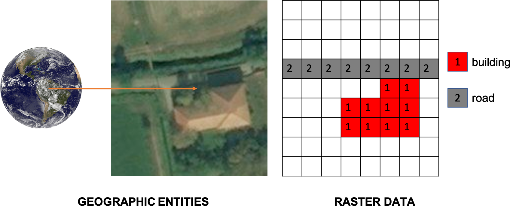
Fig. 1.3.1.1 – Schematic of geographic entities representation using the raster data model

Many raster data files, including digital satellite images, are made up of multiple matrices of pixels which are stored together into a single file. These matrices are referred to as raster bands or channels. In the case of satellite images, bands can be seen as a collection of images taken simultaneously over the same geographic area. Special satellite sensors, called multispectral cameras, measure the intensity of radiation reflected by the Earth surface in multiple regions of the electromagnetic spectrum and store measures into multiple raster bands. Through the analysis of these multiple raster bands, it is possible to infer the physical characteristics of geographic entities in an area. This is one of the main principles of the discipline called Remote Sensing that is among the most important GIS-related applications.

An intuitive example of the application of raster bands from multiple regions of the electromagnetic spectrum is the color imaging. Human eyes are able to detect radiation of three different regions of the spectrum corresponding to the red, green and blue wavelengths. Human brain combines this information into a single colour image. All the colours that are visible to humans are then created by mixing these primary colours channels. This principle is imitated by colour imaging, including digital display screens (Fig. 1.3.1.2). Multispectral satellite cameras are able to measure radiation also from regions of the electromagnetic spectrum that are not visible to human eyes. Through the combined analysis of multispectral satellite raster bands, it is possible to measure much more physical characteristics of Earth than the colour, such as surface thermal properties, vegetation conditions and the atmosphere composition. GIS offers extensive support to the analysis of multispectral raster data.

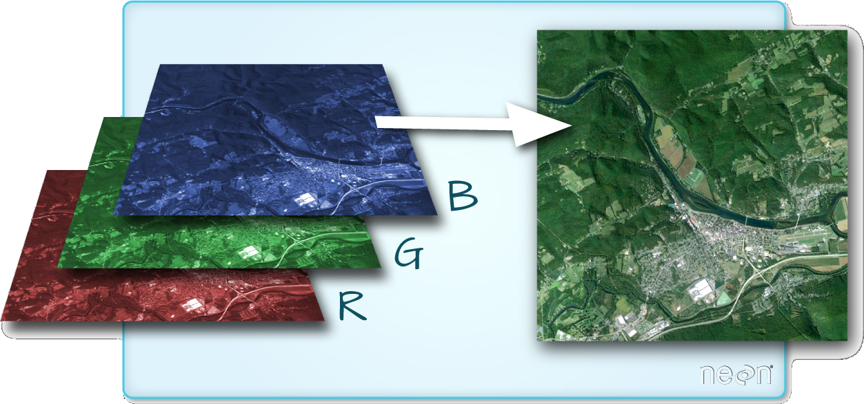
Fig. 1.3.1.2 – The principle of color imaging. Source: https://www.neonscience.org

1.3.2. Vector data

Vector data models describe geographic entities as discrete objects such as points, lines, and polygons. Point objects are recorded as single coordinate pairs, lines as ordered series of coordinate pairs while polygons as one or more ordered series of coordinate pairs where the first and last pairs coincide (close segments). Vector data attributes such as numeric values, textual information and other non-spatial characteristics of each vector object are attached to the list of coordinate pairs and linked to each specific object (Fig. 1.3.2.1). Vector data models link spatial and non-spatial elements of the data through indexes and encode them into a vector data file. Vector data can be encoded in many file formats. Some of the most popular and widely adopted vector data formats in GIS are, for example, the Shapefile and the GeoJSON.

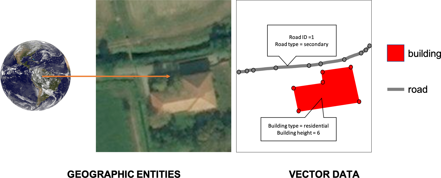
Fig. 1.3.2.1 – Schematic of geographic entities representation using vector data model

Vector data provide a sharp and scalable representation of geographic entities with almost no loss of portraying accuracy because entities boundaries are outlined directly by their coordinate values. The intuitive representation of entities provided by vector data is generally simpler to handle by users than raster data. For this reason, GIS provides many drawing functionalities to manually edit and styling vector data on maps.

The size in memory of vector data files depends mainly on the number of objects mapped in a single file and, for lines and polygons, also on the number of coordinate pairs (or vertices) that are used to describe each object. The amount and type of attributes associated with each object also influence the size. Specifically, the higher the number of vertices and attributes the better is the level of detail provided by the vector data while the data file dimension increases. Mathematical operations on vector data are generally computationally slower than raster data. This is due to the sparse or irregular object format of vector data that has to be handled by GIS software. Accordingly, the use of vector data is particularly suitable for high-detail cartographic applications focusing on a finite amount of discrete objects or involving confined geographic areas.