2.5. Raster processing

The aim of this exercise is to provide you some skills about raster data analysis and processing, starting by some very basic tools on QGIS that can help in it. During this exercise we will use the following layers that you have already been working with:

• Raster Data:

  • Land_cover
  • Temperature_distribution

• Vector Data, to be used for the overlay analysis:

  • Municipalities_OSM

Add them to QGIS from the Geopackage you were provided to your Layers panel. It is advisable to load also the raster data styles that you were given in the exercise folder (see exercise on raster visualization on QGIS) in a way to better visualize the data while analysing and processing them.

This exercise will start from some basic activities and checks that are usually taken before processing (as reprojection and removing noData) to follow then with operations and tools that can be very useful when working with raster data as Raster calculator, Vectorization, Clip and Overlay statistics. All these operations and tools can be used separately, in different order or in different ways to obtain some geospatial information from your raster data.

2.5.1. Reprojection

When you load raster data on QGIS, before starting any processing, you should look at their properties, that need to be adequate for the steps you are going to take and for the output you want to create. Here, reprojection tool can be fundamental. Indeed, raster data, as well as a whole QGIS Project, can refer to a certain map projection and, more specifically to a Coordinate Reference System (CRS) that links map locations to real places on Earth. It can happen that your raster data are referred to different CRS, and, in that case, you would not be able to compare or combine them without reprojecting them to a common CRS. Also, it can happen that the processing output needs to be referred to a CRS and so reprojection tool must be used.

A good rule is to check at the beginning the raster data CRS. It can be checked under CRS voice by going to each layer Properties → information. In this exercise, you can check that all data are referred to “CRS: EPSG:32632 - WGS 84 / UTM zone 32N – Projected”. Therefore, we would not need to do any reprojection.

However, to learn how to reproject data, let us apply reprojection to Land_cover. Look at Fig. 2.5.1.1 to follow with numbers in brackets the different steps that here will be mentioned.

To start, go to Raster Menu on QGIS → Projections (1) → Warp (Reproject) (2): it will open the Warp (Reproject) window. There, you need to set the input layer (Land_Cover) (3), with its input CRS (Project CRS: EPSG:32632 - WGS 84 / UTM zone 32N) (4) and the final desired CRS, the target CRS (here choose EPSG: 2056-CH1903+/LV95) (5). Leave the rest as it is and click on Run to reproject the raster in a new CRS. To choose the target CRS, by clicking on the icon (5), after having unchecked No CRS box (6) in the new window, you can search for the wanted target CRS (7): as in Fig. 2.5.1.1 (7) search for EPSG: 2056 and then select the option for the swiss Obl. Mercator projected CS (8).

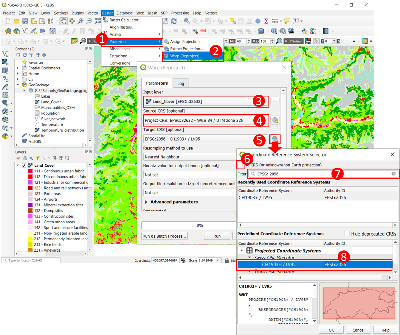
Fig. 2.5.1.1 – Raster data Reprojection steps.

The new added raster, called reprojected is a temporary File. This reprojected File still perfectly overlaps with the original one, even though the two layers have different CRS. This is because QGIS_3 automatically applies “on the fly” CRS transformation for both raster and vector data. This means that, for visualization, layers with different CRS are transformed into the project’s CRS (here the EPSG:32632 - WGS 84 / UTM zone 32N) provided that the input layers CRS is stored in their metadata and that it is correct. Thus, to see the CRS change you can go to reprojected layer Properties → Source and change its source CRS: in this way, you won’t see anymore the reprojected File together with the original one, and, to visualize it, you will have to Zoom to its extent. That is because now QGIS has no more reprojected it ‘on the fly’ and you can see therefore the effects of referring to a different CRS.

2.5.2. Removing NoData

Go back to the original Land_Cover layer on which you have applied the Land_Cover_style, provided to you in the exercise folder. As already noticed during the Raster visualization on QGIS exercise, this style contains more classes and values than the ones really present in this area, because it was created for the whole Corine Land Cover map that is much wider than this portion we are referring to. Particularly, the Land_Cover_style 999-NODATA class, corresponding to value 48, is not present in our area under study, you can check it by visualizing the raster with Singleband-grey render type, to see it contains no pixels with value 48. Therefore, you can remove this class visualization from Land_Cover_style, by clicking on minus icon (Fig. 2.5.2.1, (2)) and you can re-save the style.

There is another huge difference when visualizing this raster with Singleband-grey render type: the Land_Cover layer contains pixels with 0 value that are no more visible when loading again the Land_Cover_style. See Fig. 2.5.2.1 to follow the steps to visualize them also with the Land_Cover_style: use the + button (3) in the Properties → Simbology window, to add a new class to be visualized: by assigning to it value 0, NoData label and an evident color as black (4), you will see again, on borders, black pixels with 0 value that will appear also with this Land_Cover_style.

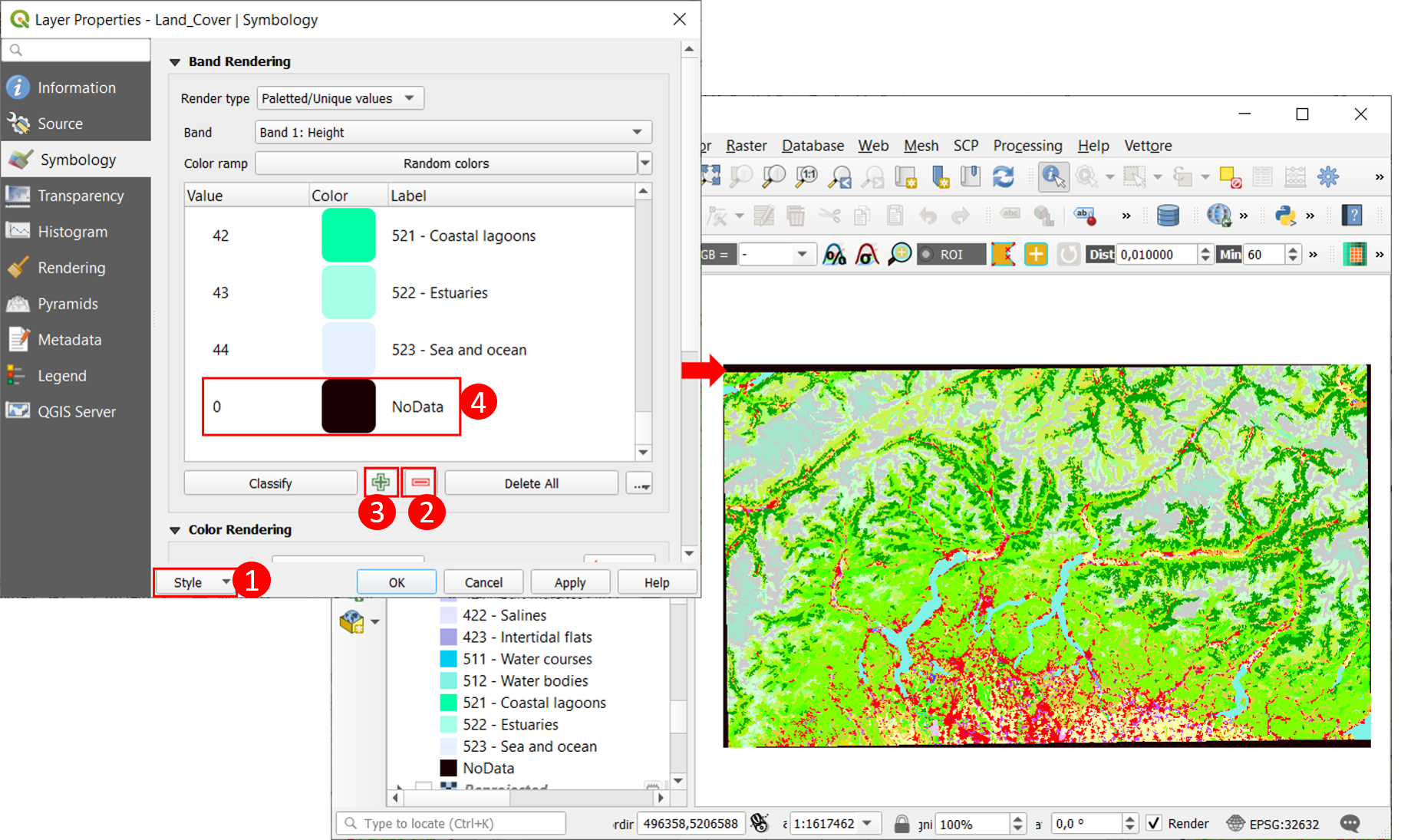
Fig. 2.5.2.1 – Visualize NoData pixels on the Land_Cover_style.

These black pixels are due to a previous conversion from Coordinate Reference System to a projection, during which they have remained empty. It is preferable to change their 0 value with null value, in a way to exclude them from following calculations. See on Fig. 2.5.2.2 the operations to be made. Go to Processing Toolbox (1) → GRASS → Raster → r.null (2) and open r.null window where it is requested the raster map for which to edit null values (3) (Land_Cover [EPSG:32632]), the list of cell values to be set to null (4) (here type 0) and finally where to save the new raster file. By clicking on Run, a new raster will be created without the 0 value pixels.

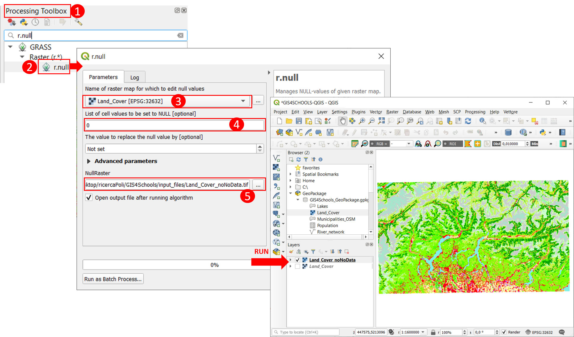
Fig. 2.5.2.2 – The steps to remove NoData pixels.

2.5.3. Raster calculator

The Raster Calculator tool allows to perform calculations based on the raster pixel values. Calculations are computed on each pixel value and the result is a new raster whose pixel values are the corresponding results from calculations on the corresponding pixels. It is a great tool that can be useful for several applications and for very different operations to apply.

Let us apply it on Temperature_distribution raster data. Before, remove NoData from this layer by applying r.null on it, setting to null its nan values (stored in the pixels among the lakes). Save this layer as Temperature_distribution_null.

Suppose that we want to find out the areas in the lakes with the lowest water surface temperatures. First, look at the distribution of values in the raster: the highest detected temperatures are obviously distributed along the borders of the lakes and are fewer with respect to the lower temperatures in the centre of the lakes. It is possible to look also at the raster data histogram (Properties → histogram) to see that the most of values are around 12,5°, thus, to find out where the lowest temperatures are localised, let us consider 12° as temperature of reference.

Now, apply Raster Calculator. See Fig. 2.5.3.1 for the steps. Under Raster Menu go to Raster Calculator…: it will open a window where to insert the following operation (1) to be performed:

("Temperature_distribution_null@1"< 12 )  * 1 + ("Temperature_distribution_null@1" >= 12 ) * 2

Particularly, with Raster Calculator, it is recommendable to insert the different signs and layers through Operators and Raster Bands buttons.

Our operation is mostly of a logical type (using < and >=): in QGIS, the results of a logical formula can be 1=True or 0=False: therefore, when we input, for example, (Temperature_distribution_null@1”< 12)* 1 the result here will be 1 or 0 for each pixel, summed to the result of (“Temperature_distribution_null@1” >= 12 ) * 2 that will be 0 or 2. Obviously one number cannot be contemporarily < or >= 12 therefore the whole result will be 1 or 2. Before running the computation insert in (2) where to save the new raster layer: when choosing for the name of the new raster you can use lowest_temperatures.

After running, a new raster layer will be added to your QGIS project. After changing its render type to Paletted/unique values, you should get a result similar to the one in Fig. 2.5.3.1 with pixels with only 1 and 2 values.

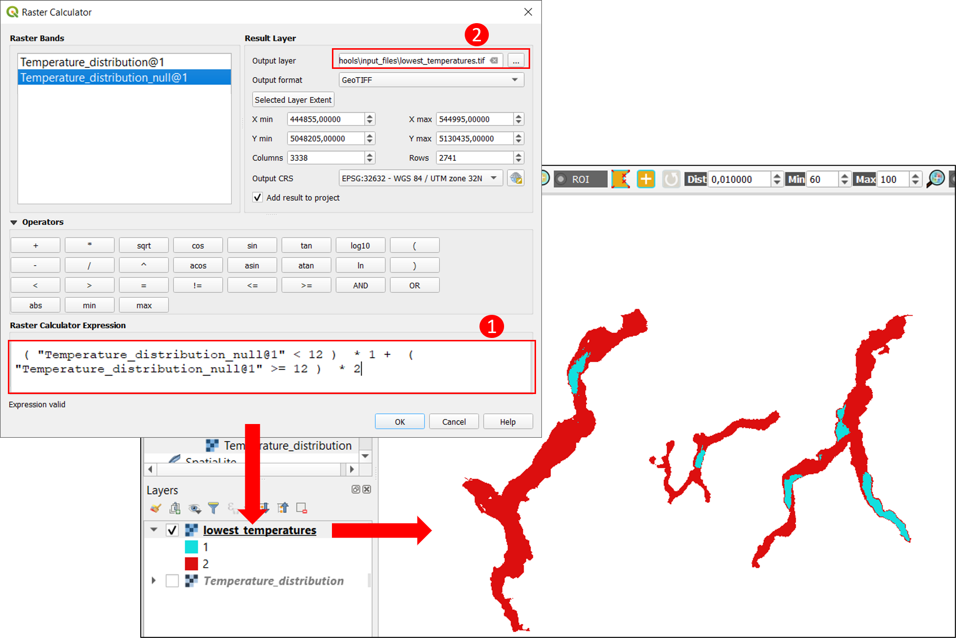
Fig. 2.5.3.1 – Raster Calculator steps and result.

2.5.4. Vectorization

The following exercise will be performed on the lowest_temperatures layer, the raster resulting from the previous Raster Calculator exercise. Vectorization is the operation to convert a raster layer into a vector one, particularly here into a polygon one.

See Fig. 2.5.4.1 to follow with the instructions. Go to Raster Menu → Conversion → Polygonize (Raster to Vector). In Polygonize (Raster to Vector) Window enter the Input layer (1) (lowest_temperatures),the name of the attribute field to create related to the raster values (2) (Low-notLow) and finally where to save the vectorized File (here named as TemperaturesLow_notLow) (3). Finally, the result will be a polygon layer. As you have already learnt in the exercise of Vector Visualization, change the polygon style into a categorized symbolisation, hide polygon symbol for ‘other values’: you will get the layer visualization that you can see at the end in Fig. 2.5.4.1.

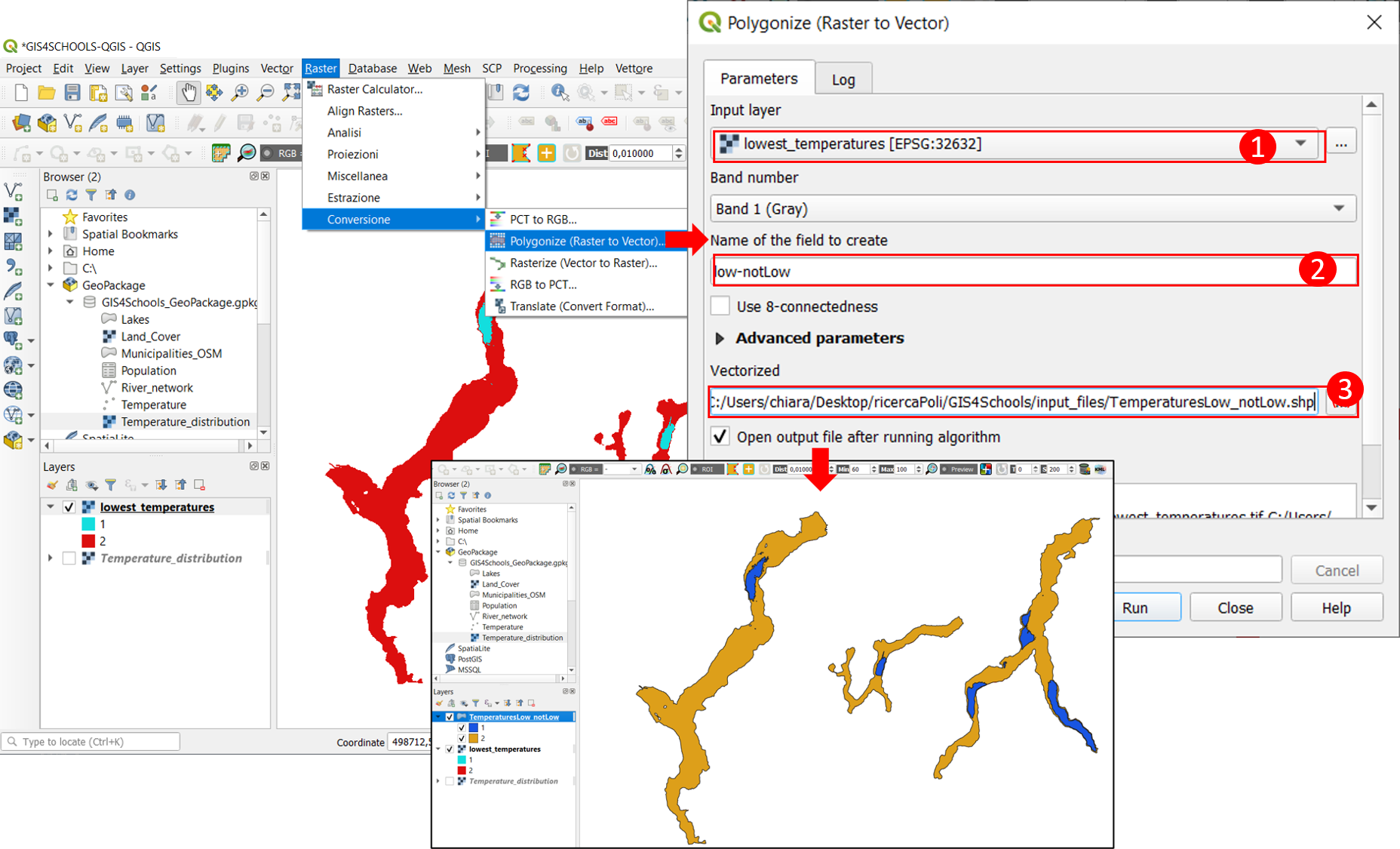
Fig. 2.5.4.1 – Vectorization steps and result.

2.5.5. Clip raster with a mask, clip raster by extent

Sometimes raster data cover a wider area than the one under study, thus, data can be much heavy and processing slowed down. In this case, it is always advisable to reduce the raster extent by clipping out the area that is not under study. There are more ways to do it, in this exercise we will focus on clipping with a mask (using another layer as reference) and on clipping by extent (taking as reference a manually drawn area).

Consider the temperatures_distribution layer. Suppose you want to study only the Maggiore lake area: it is possible to clip the temperature_distribution layer by a manually rectangular drawn region that would exclude the other two lakes. Refer to Fig. 2.5.5.1 to follow on with the instructions. Go to Raster Menu → Extraction → Clip Raster by Extent…. It will open a window where to input the layer to be clipped (1) (Temperature_distribution) and the clipping extent: click on … button (2) and then on Draw on Canvas (3) to manually draw on your project the clipping area, a grey rectangle on Maggiore lake (4). Then, for this exercise, just save it as temporary File, Run and the result will be the layer of temperatures cropped just on the Maggiore lake.

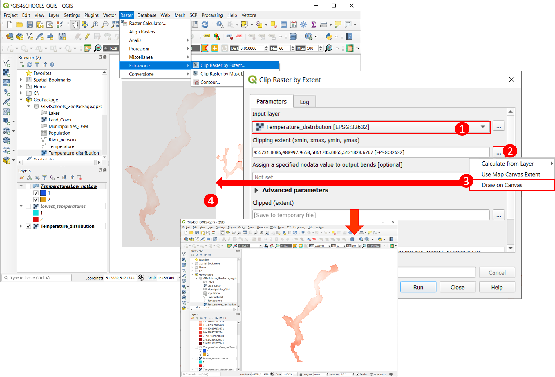
Fig. 2.5.5.1 – Clip Raster by extent, steps and result.

Now, on the other hand, let us see how to clip a raster with a mask. When clipping with a vector mask it is possible also to decide which categories of the polygon vector to be used to mask the raster data. Suppose here we want to mask the temperature_distribution layer for where its temperatures are the lowest, thus where the TemperaturesLow_notLow polygons have value 1. Click on Select Features by value and set low_notLow field equal to value 1, to select the polygons with the lowest temperatures. Then, go to Raster Menu → Extraction → Clip Raster by Mask Layer…, input layer: Temperature_distribution, to be masked by TemperaturesLow_notLow vector layer, check the Selected Features only box (to mask the raster with just the selected polygons of the mask layer) assign 0 as NoData Value and Save to a temporary File. In the end, the new added layer should cover with temperature values, only the areas of low water surface temperature.

2.5.6. Overlay statistics

Raster data allow to easily compare and combine different data referred to the same territory. In this way, they allow also to easily compute overlay statistics that can be a powerful tool to investigate some areas. Zonal statistics algorithm is an example of the overlay statistics that can be computed from the combination of a raster and a vector layer. This tool, from raster data, calculates statistics (e.g. mean, max, min…) for each feature of the overlapping vector layer.

To better understand it, suppose that we want to know the municipalities with the coldest or hottest surface water temperatures. By overlapping the vector layer Municipalities_OSM to the Temperature_distribution raster, lakes areas are subdivided in smaller portions according to the municipalities they are part of. Therefore, it could be possible to derive some statistics for each of these portions of lakes.

See Fig. 2.5.6.1. Go to the Processing Toolbox → Raster Analysis → Zonal statistics insert as input layer the Municipalities_OSM vector (1) and as raster layer the Temperature_distribution raster (2). Then name the Output column prefix LakeTemp (3) and select the statistics to calculate (here mean, max and min), by clicking on the “…” button (4). By saving to a temporary File, the algorithm will add to QGIS a new vector layer, similar to the Municipalities_OSM, containing in its Attribute Table three new columns (fields), one for each calculated statistic. To check the results, click on LakeTempmean column to sort features from the highest to the lowest value: you should find that it is Melide municipality the one with the highest mean lake surface temperature (22°) while Valmadrera is the one with the lowest lake surface temperature (11,7°) on the same day.

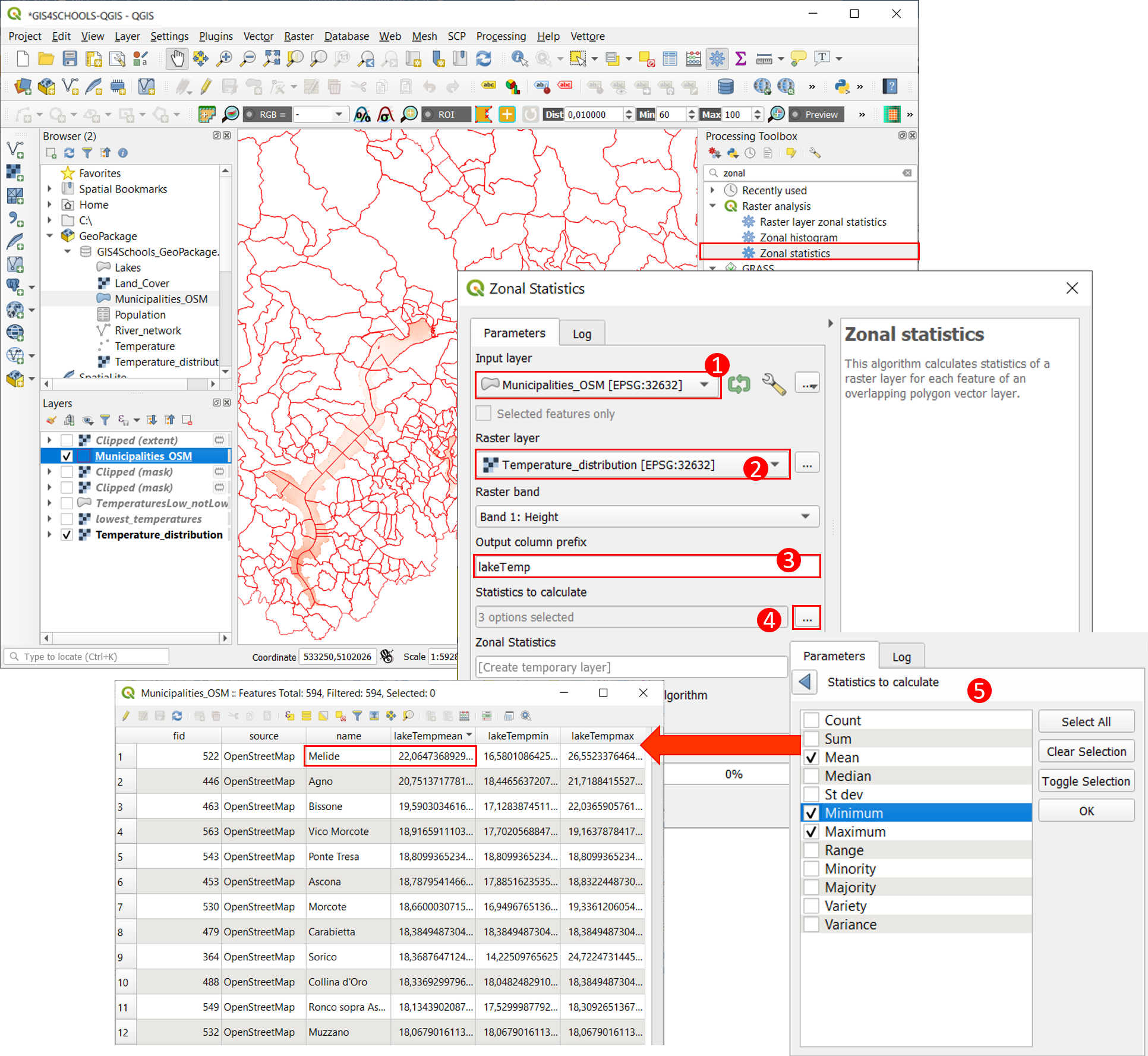
Fig. 2.5.6.1 – Zonal Statistics algorithm, steps and result.

Try to do it also on the single Maggiore lake temperature distribution layer that you have cut in the previous exercise (clip by extent) to get the municipalities with the highest or lowest mean temperature for just that lake area.