2.4. Vector processing

In this lecture we will introduce some common tools available on QGIS for the analysis and processing of vector data. QGIS provides different functions for the management and analysis of vector data, such as tools for map digitizing, features research and selection, editing and geoprocessing. We are going to use the following vector files:

• Lakes.shp (polygons representing the main lakes of the area of interest);
• River_network.shp (lines representing the river network across the lakes basins);
• Municipalities_OSM.shp (polygons representing the boundaries of the municipalities);
• Temperature.shp (points representing the lakes surface water temperature).

2.4.1. Map digitizing

One of the most common activities that a GIS user has to carry out is map digitizing, that consists in converting raster data (such as digital maps) in vector data that can be used for different analyses. Assume that the aim is to digitize a lake and a water course in the area of interest, therefore to add two different features to the existing layers Lakes and River_network. Let us consider Standard OpenStreetMap as a basemap for digitizing the two features. In this case, in the main menu of QGIS, let us select Web → QuickMapServices → OSM → OSM Standard [1] and zoom to the area of interest (North Italy and Switzerland, among Lakes Maggiore, Como and Lugano). Then, let us open the two layers that have to be updated. In the top menu select Layer → Add Layer → Add Vector Layer (this is the general way to open a vector file in QGIS). Select the shapefile Lakes.shp and River_network.shp in the folder that contains all the data (specifying as file format ESRI Shapefiles) and then click Add. For a better visualization of these elements, let us change the symbology of lakes and rivers by assigning them the same colour, for example light blue.

Now, let us zoom to the area around Lecco: the aim is to digitize Lake Garlate and Lake Olginate, which can be easily identified through OpenStreetMap (they are south of Lecco). For this purpose, let us open the Digitizing Toolbar by right-clicking on the grey area that contains all the tools provided by QGIS and checking both Digitizing Toolbar and Advanced Digitizing Toolbar. In order to enable all the digitizing tools, let us start an editing session: right-click on the layer Lakes and click Toggle Editing. The Digitizing Toolbar is now enabled (Fig. 2.4.1.1). Click Add Polygon Feature on the Digitizing Toolbar and manually draw Lake Garlate and Lake Olginate simply by adding every vertex of the polygon (with a left click of the mouse). When a polygon is complete, that is, all the vertices have been added, right-click the last vertex (1); then, adequately fill the layer fields (2) (for example, for Lake Garlate write “Lago di Garlate” in the field Name and “OpenStreetMap basemap” in the field Source) and click OK (3) (Fig. 2.4.1.2). Continue to digitize in the same manner the other lake.

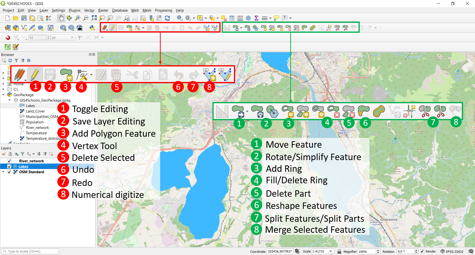
Fig. 2.4.1.1 – Digitizing Toolbar and Advanced Digitizing Toolbar.

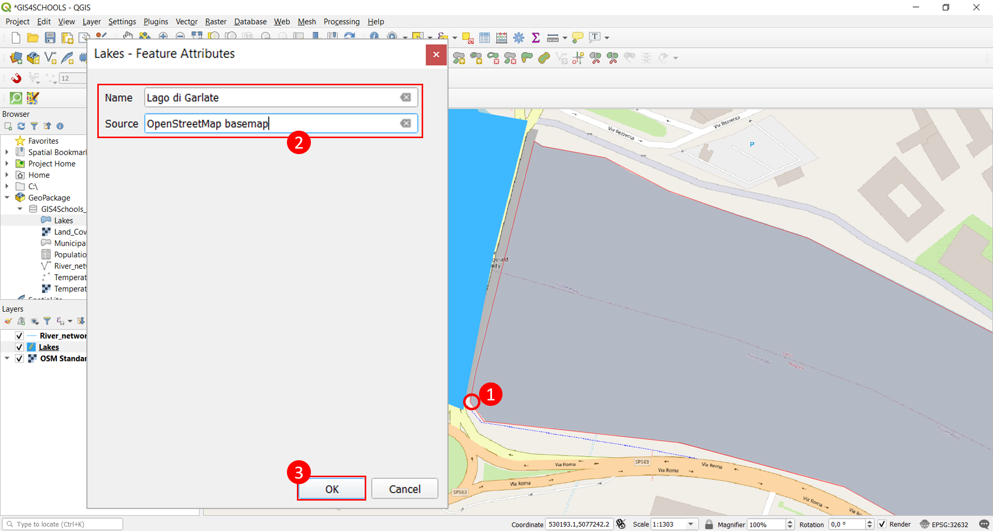
Fig. 2.4.1.2 – Polygon feature digitizing.

In order to digitize an island, we can use the Add Ring function of the Advanced Digitizing Toolbar after selecting the feature that contains the island (Fig. 2.4.1.3). This function allows the creation of a hole in a polygon feature (for example, Lake Garlate contains an island called Isola Viscontea, as shown in Fig. 2.4.1.3). First, select the polygon to be modified (1), then click on the Add Ring button (2) and digitize the ring, right-clicking when it is complete (3).

Fig. 2.4.1.3 – Ring digitizing to create a “hole” within a polygon feature.

As Lake Garlate and Lake Olginate are divided by a dam, we could digitize a single polygon that contains both lakes and then split the feature into two parts using the Split Features tool (available in the Advanced Digitizing Toolbox). For this purpose, we have to select the feature that has to be divided and then digitize the line of separation with the tool Split Features (as always, right-clicking when the line is complete). Similarly, we can merge two parts of the same feature by selecting the two parts and using the tool Merge Selected Features.

Imagine that we have made a mistake in the digitizing procedure and we want to reshape a feature. In this case, we have to select the feature that has to be modified (1) and use the Reshape Features tool (2). It is simply necessary to redefine the feature boundary where the error is present, digitizing the correct line and right-clicking when it is complete (3) (Fig. 2.4.1.4). Alternatively, we can redefine the boundary with the tool Split Features, selecting the part that has to be deleted and using the tool Delete Part. Another possibility consists in changing directly the position of the vertices, with the Vertex Tool (current layer): it is simply necessary to click on the vertex that has to be moved and click again on the right position.

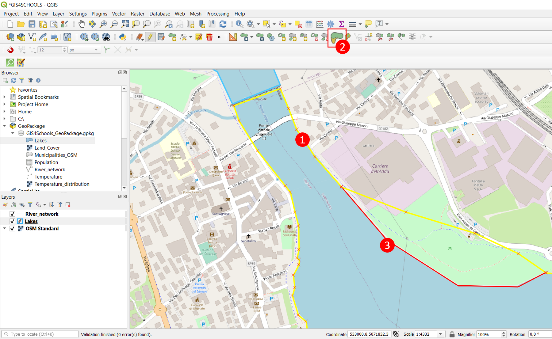
Fig. 2.4.1.4 – Reshape feature tool.

Once the features have been correctly digitized, we need to save (clicking on Save Layer Edits) and stop the editing session (clicking on Toggle Editing again).

A similar procedure applies to linear features. Let us consider the layer of rivers (River_network). In this case we are going to digitize a short tributary of Lake Como. Let us zoom in the area of Como (and in particular the area of Germanello) with the help of the basemap. The aim is to digitize the water stream called Torrente Caraello. Toggle editing on the River_network layer and click Add Line Features (1). The line can be created by clicking the position of every vertex and then right-clicking when the line is complete (2). As seen with polygon features, the user has to fill the attributes (3) that characterize this feature (Fig. 2.4.1.5) and then click OK (4). The same tools introduced for polygon features can be used for linear features as well (Split Features, Reshape Features, Merge Selected Features and Vertex Tool). Once again, when the feature has been created, we have to save and stop the editing session.

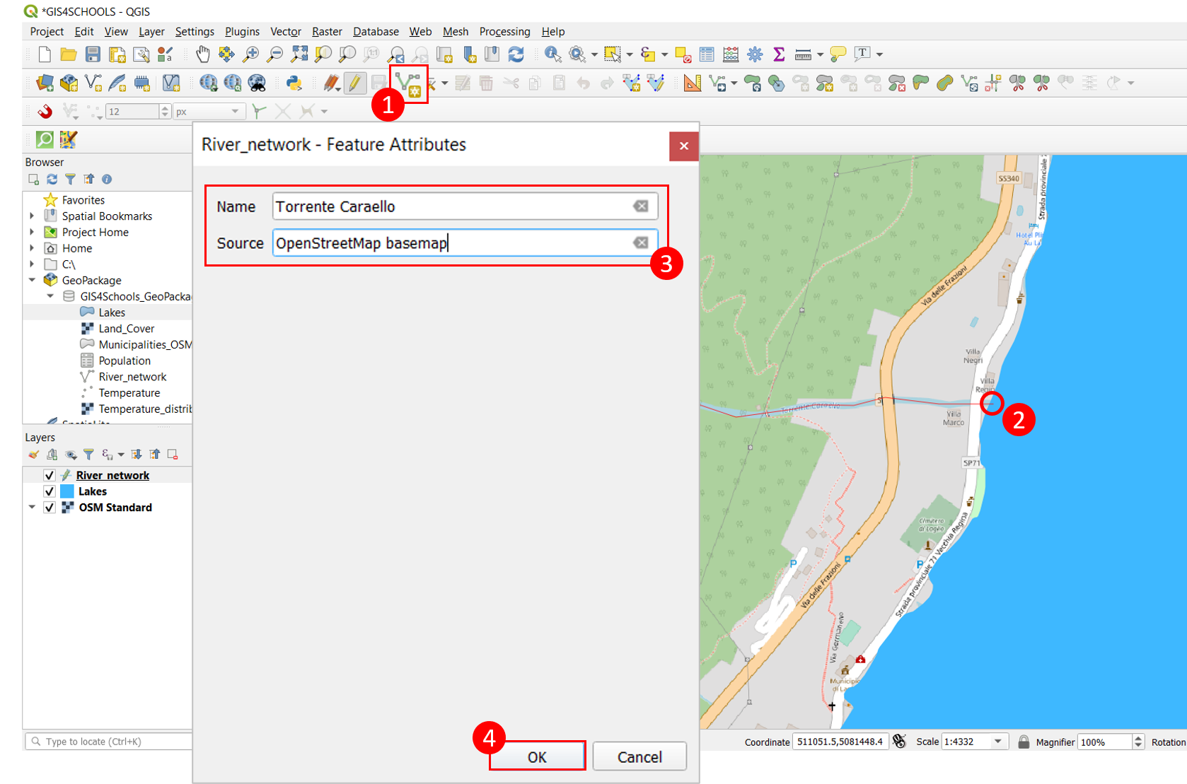
Fig. 2.4.1.5 – Polyline feature digitizing.

[1]	If the QuickMapServices plugin is not installed, select from the top menu Plugins → Manage and Install Plugins, search for QuickMapsService and select Install Plugin.

2.4.2. Attribute table: selection, editing and field calculator

In this section we are going to look at the attribute table of some vector data. We are going to describe how to select the features constituting the vector layer, how to edit them and how to use the field calculator. For this purpose, let us open the shapefiles Municipalitis_OSM.shp and Temperature.shp with the same procedure described in the previous paragraph.

It is possible to identify a feature belonging to a single layer by selecting that layer in the Table Of Contents and using the tool Identify Features (1) in the top menu. In this way, if we click, for instance, on Lake Maggiore (2), a window on the right opens (3) and the attributes of that feature are displayed (Fig. 2.4.2.1). The information provided are those contained in the attribute table. As shown in Fig. 2.4.2.1, the selected feature is displayed in purple.

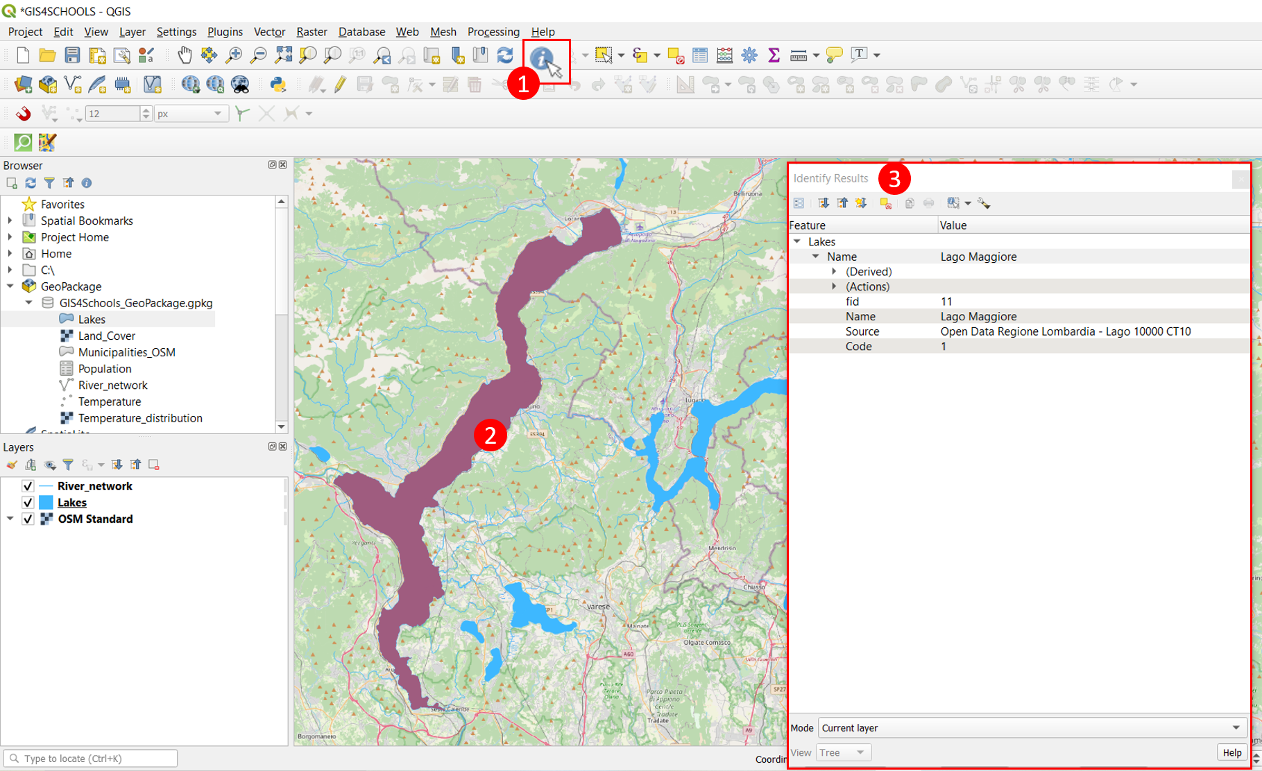
Fig. 2.4.2.1 – Feature identification (Lake Maggiore).

Let us now look more in detail at the attribute table of the Lakes layer. To open the attribute table, right-click on the layer and click Open Attribute Table. The attribute table is organized in columns and every column corresponds to a field (in this case, the layer has two textual fields, namely Name and Source). Every geometric feature (row) is associated with semantic information called attributes. Fig. 2.4.2.2 shows the attribute table of the layer Lakes.

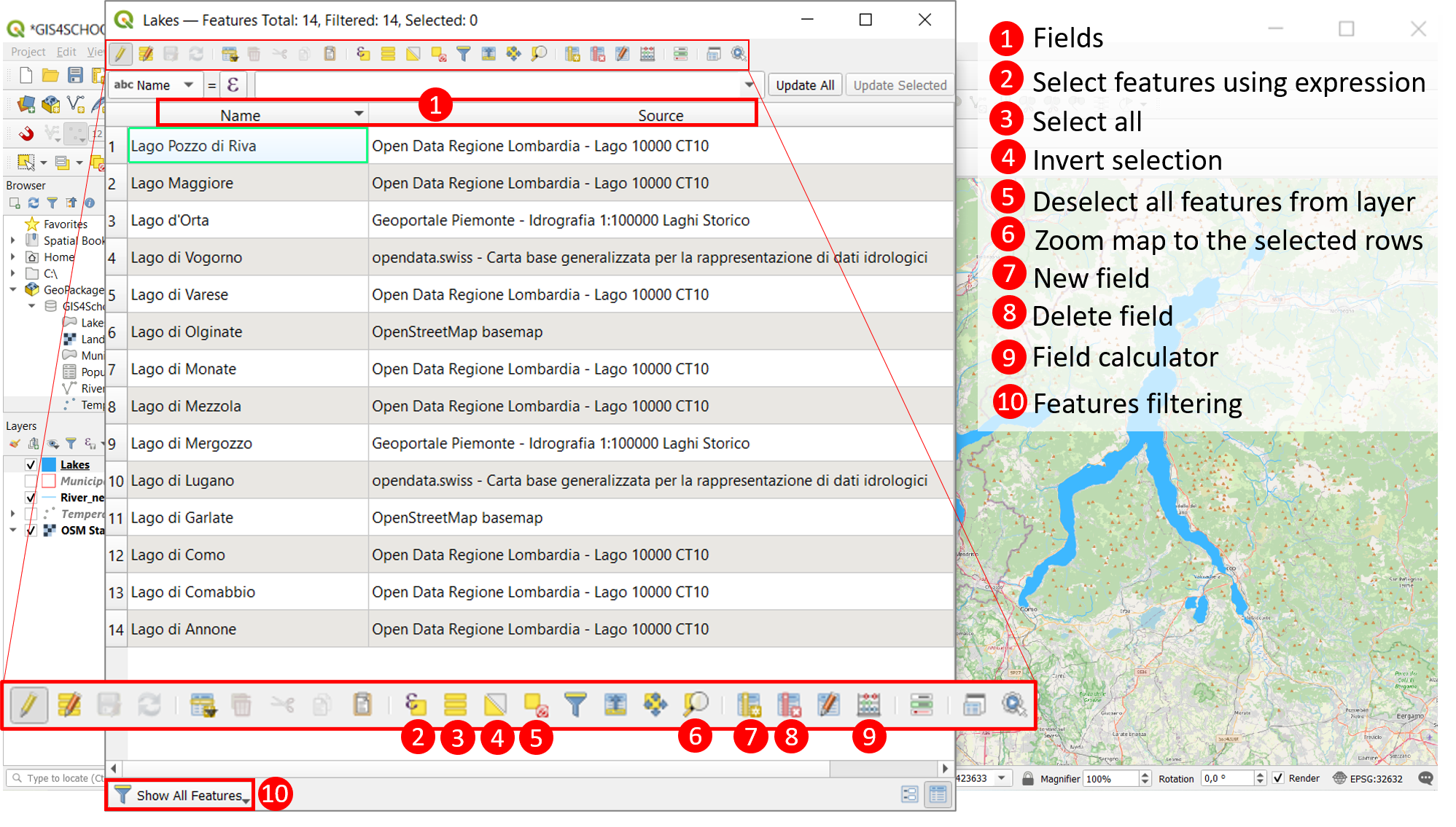
Fig. 2.4.2.2 – Attribute table of the layer Lakes.

Suppose that we want to add a new field that indicates the area covered by every feature. First, we need to start an editing session (right click on the layer Lakes → Toggle Editing or, if the layer attribute table is open, directly click on Toggle Editing (1) on the top menu of the table). Afterwards, click the tool New field (2) in the table top bar and provide the field name and type: in this case, let us call the field Area and assign the type “decimal number (real)”. In order to calculate the area, we have to use the Field Calculator (3) that is available in the main menu of the attribute table (look at Fig. 2.4.2.3). Check the option Update existing field (4) and select the field Area (5). In the Expression tab, expand the section Geometry and double click $area (6). Clicking on OK (7), the area (in square meters) of every geometric feature is calculated and reported in the corresponding line of the attribute table under the field Area. Fig. 2.4.2.3 shows the procedure just described.

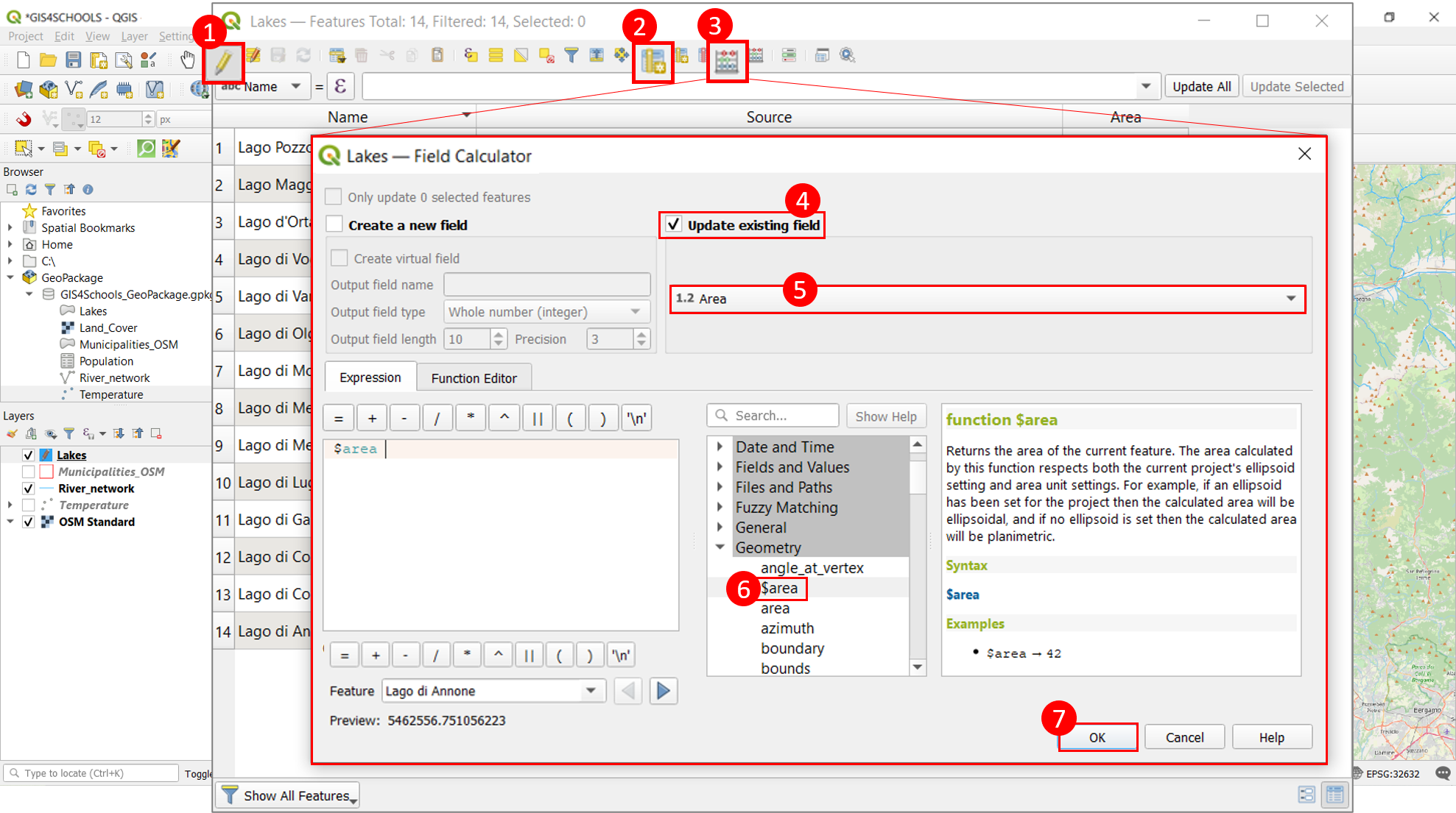
Fig. 2.4.2.3 – Computation of polygon features area through the Field Calculator.

It is also possible to modify a single attribute simply by clicking the cell that has to be updated and typing the new attribute. Furthermore, it is possible to update the attributes of a specific set of features. In this case it is necessary to select these features (clicking the corresponding line number in the attribute table) and use the field calculator, as previously explained: only the attributes of the selected features will be modified. Once again, it is necessary to save and stop the editing session with the usual procedure.

Now we are going to see different ways to select geometric features. In particular, we will describe the following possibilities: selection by geometry, selection by expression and selection by location. For this purpose, it is quite helpful the Selection Toolbar, that can be enabled by right-clicking on the grey area of the QGIS main menu. The procedures that are going to be described are synthesized in Fig. 2.4.2.4 and Fig. 2.4.2.5.

• Selection by geometry (Fig. 2.4.2.4, left button): the simplest way to select a feature is to select it directly in the map. This type of selection can be performed through the tools Select Feature (or Select Features by Polygon, by Freehand and by Radius). In this case, it is necessary to select the layer of interest in the Table of Contents. When the feature is selected, it turns to yellow in the map.
• Selection by expression (Fig. 2.4.2.4, central button): it is possible to select feature elements with an appropriate expression. All the features that meet the conditions written in such expression are selected. For instance, we can select all the features of the layer Lakes having an area greater than 10⁷ m² and coming from the Lombardy Geoportal (Source field). Similarly, we can select features by value: a guided interface allows us to specify the value of the layer fields. It is also possible to select all the features of this layer (Select All Features) and to invert the current selection (Invert Feature Selection). Furthermore, it is possible to deselect all features belonging to all layers (Deselect Features from All Layers) or to deselect all features belonging to the currently active layer (Deselect Features from the Current Active Layer), as shown in Fig. 2.4.2.4 (right button).

Fig. 2.4.2.4 – Features selection through the Selection Toolbar.

• Selection by location (Fig. 2.4.2.5): this selection possibility allows to select the features that respect certain spatial characteristics. For example, we can select all the municipalities that intersect the lakes. Click Vector → Research Tools → Select by Location (1) and specify the following parameters: select features from Municipalities_OSM (2), where the features intersect (3), by comparing to the features from Lakes (4). Finally, click Run (5).

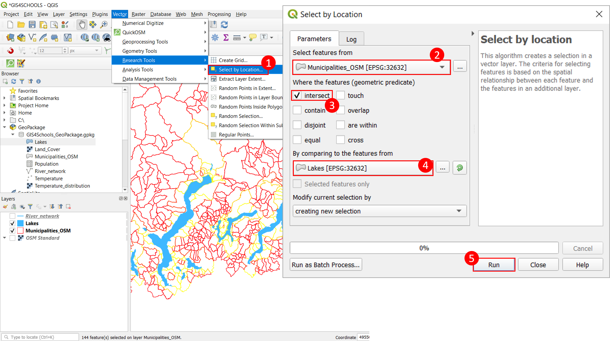
Fig. 2.4.2.5 – Selection by location.

Once the selection has been performed, we can export the selected elements and save them in another layer. For example, let us extract the municipalities that intersect the lakes (i.e. the last selection that we have performed) in another shapefile. It is necessary to right-click on the layer Municipalities_OSM and select Export → Save Selected Features As. We have to specify the format ESRI Shapefile, the file name (for example, Municipalities_on_lakes) and click OK. The new layer will be automatically uploaded in the QGIS project and displayed in the map.

2.4.3. Join

Not all the data that can be used in a GIS environment are strictly geospatial. Tabular data without direct geospatial references may be used as well, but they have to be linked to other geospatial data through a join operation. A join operation establishes a 1 to 1 relationship between the rows of the tabular data and the rows of the vector data attribute table. In order to create a join, the user has to identify a field, called key, that exists in both tables and on which the correspondence is based.

The table Population.csv contains the number of inhabitants of all the municipalities around the lakes. Let us suppose that we want to add this information to the existing shapefile Municipalities_on_lakes.shp (that we have previously created). In this case, the key is represented by the municipality name that exists in both files.

First, we have to add the table to the QGIS project (look at Fig. 2.4.3.1). Select Layer → Add Layer → Add Delimited Text Layer (1). Specify the table path (2), check the option Custom delimiters (3), Others and type “;” (4). Check First record has field names and Detect field types (5). Check No geometry (attribute only table) (6). Finally, click OK (7). Once the table is added, we have to create the join. All the steps are shown in Fig. 2.4.3.2. Right-click on the layer Municipalities_on_lakes and click Properties. In the tab Joins (1), click the button Add new join (plus symbol) (2) and set the following parameters (3). Join layer: Population (table), Join field: NOME_COM, Target field: Name. Click OK (4) and then OK again (5).

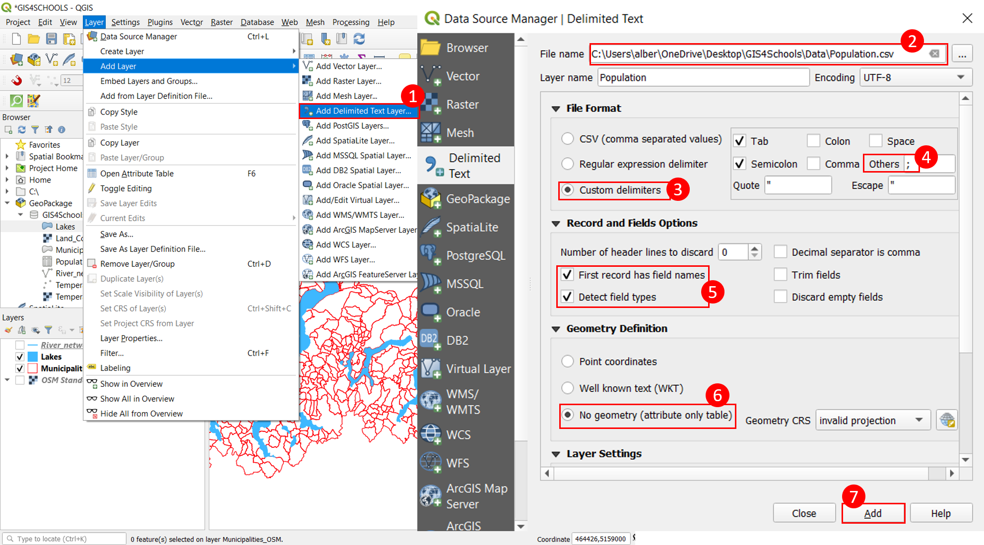
Fig. 2.4.3.1 – How to add the tabular file Population.csv in QGIS.

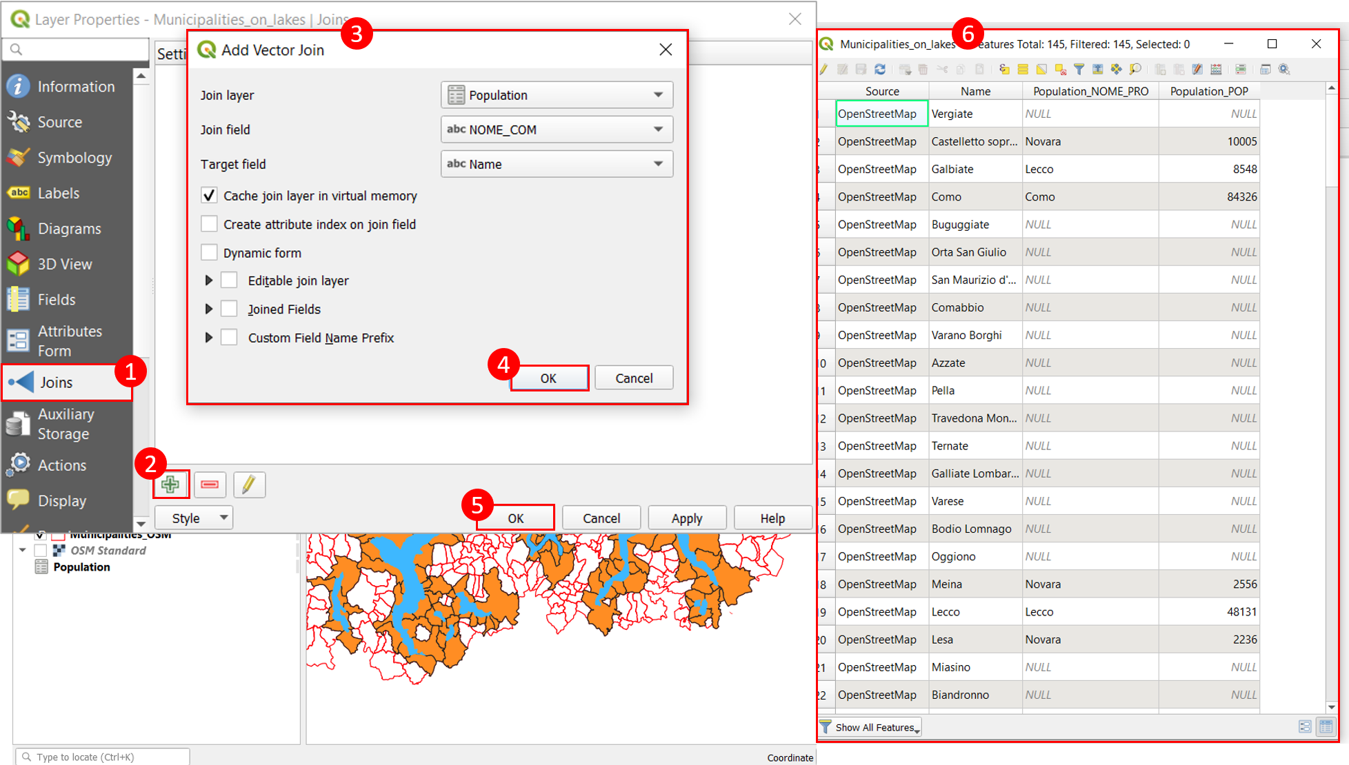
Fig. 2.4.3.2 – Join between Municipalities_on_lakes.shp and Population.csv.

As a result, the fields of Population.csv have been added to the attribute table of Municipalities_on_lakes.shp (6). As shown in Fig. 2.4.3.2, in some cases there is no correspondence between the names of the municipalities in the two files, therefore we find the value “NULL” in the cell. This is due to the fact that the information comes from different sources and in particular the table Population.csv only regards the municipalities around Lakes Maggiore, Como and Lugano (while the other file also regards other lakes, like Lake Varese). In most cases the correspondence exists anyway.

It is very important to highlight that join is a temporary operation and it does not change the original data. This means that if we want to save the joined table, we have to export it into another shapefile: click on the layer Municipalities_on_lakes → Export → Save Features As. Let us call the new shapefile Municipalities_on_lakes_pop.shp and save it in the folder that contains all the other data.

If we open the attribute table of this shapefile (Municipalities_on_lakes_pop.shp), we can see that the fields coming from the join operation with the table Population.csv do not have appropriate names. These names have been assigned by default by QGIS, but it is preferable to change them for the next steps.

In particular, the field containing the number of inhabitants of each municipality is called Populati_1 and the field containing the province is called Population. In order to change the name of these fields, we can use the tool Refactor Fields: in the Processing Toolbox (gear symbol in the top menu of QGIS), search for Refactor Fields and double-click to open the configuration interface.

Select as Input layer Municipalities_on_lakes_pop (1); change the name of the fields Population (Text) and Population_1 (Whole number), respectively, into Province and Population (2). Then, choose an adequate path for the output and call it Municipalities (3). Finally, select Run (4). Fig. 2.4.3.3 shows the procedure just described.

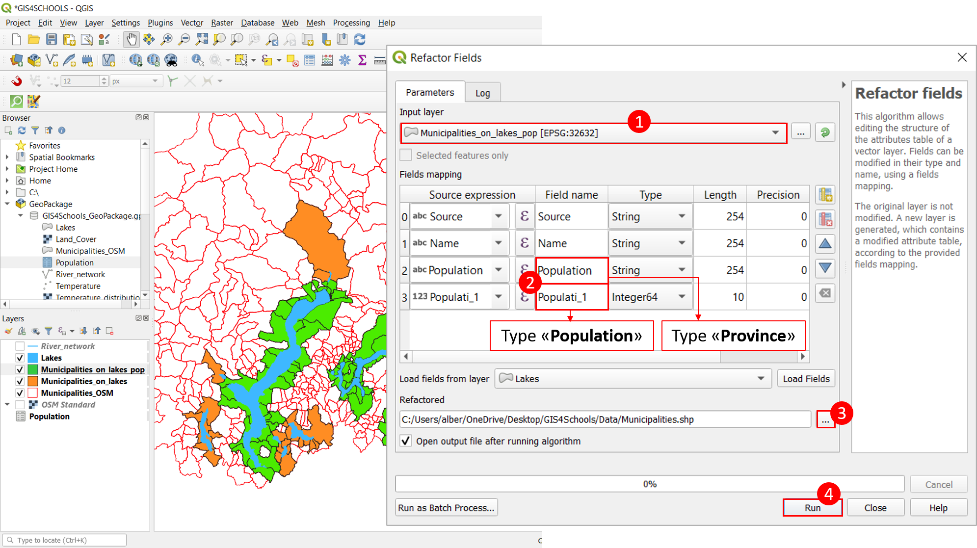
Fig. 2.4.3.3 – Configuration interface of the tool Refactor Fields, that allows to change, for instance, the fields name of an attribute table.

2.4.4. Geoprocessing tools for vector data: dissolve

In this part of the lecture we are going to explore some useful geoprocessing tools that are available in QGIS. All the geoprocessing tools for vector files can be found in the main menu, under Vector → Geoprocessing Tools. The same tools are available in the Processing Toolbox (main menu → Processing → Toolbox). In this lecture we will describe three important tools: dissolve, intersect and buffer.

The dissolve tool allows the user to combine different elements of the same layer based on the value of a certain field. The elements (features) that have the same value for that field are merged. Suppose that we want to apply this tool to the layer Municipalities, in order to merge the municipalities belonging to the same province.

First of all, let us remove the features coming from the shapefile Municipalities_on_lakes.shp that did not have any correspondence with the rows of the table Population.csv. Let us open the attribute table of the layer Municipalities and start an editing session (Toggle editing mode on Municipalities). Click on Select features using an expression and type the expression “Population is null”. Click OK. Then, click Delete selected features. Save and stop the editing session.

Now, click on Vector → Geoprocessing Tools → Dissolve (1). Select as Input layer: Municipalities (2). Select Dissolve field: Province (after clicking on the ellipses symbol) (3). Save the Dissolved layer, namely Municipalities_on_lakes_diss.shp, in the usual folder (4). Finally, click Run (5). Fig. 2.4.4.1 summarizes the procedure and shows the result.

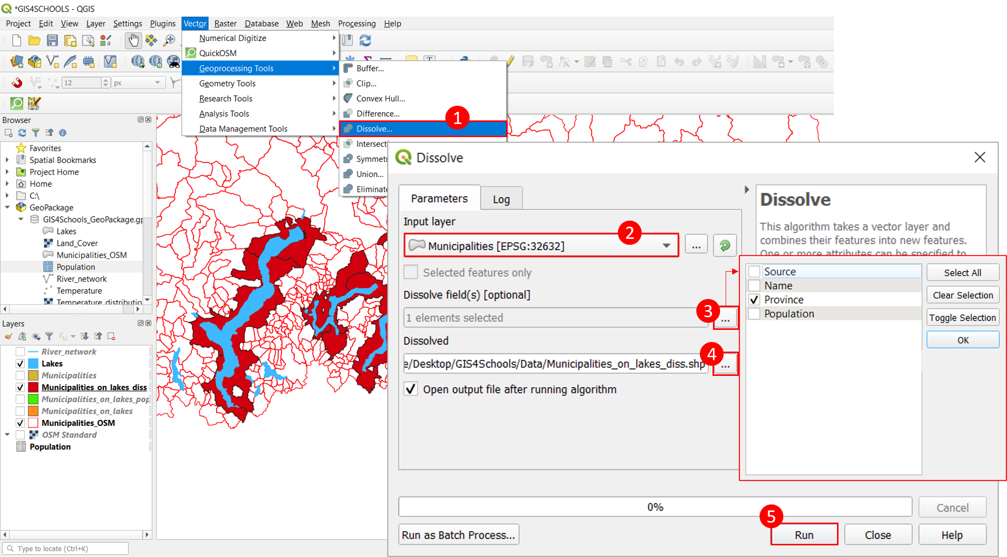
Fig. 2.4.4.1 – Dissolve configuration interface: procedure to follow. The result of the dissolve operation is shown: Municipalities_on_lakes_diss (dark red polygons).

2.4.5. Geoprocessing tools for vector data: intersection

The tool intersection extracts the overlapping portion of features belonging to two different layers. Features in the output layer are assigned the attributes of the overlapping features from both input layers. In this exercise we are going to extract the portions of rivers that are within the lakes’ boundaries. Indeed, the points of intersection between rivers and lakes are particularly delicate and important from an environmental point of view.

Select Vector → Geoprocessing Tools → Intersection (1). Select as Input layer River_network (2) and as Overlay layer Lakes (3). Then, save the new shapefile (Intersection), with the name River_lakes_intersect.shp in the usual folder (4). Finally, click Run (5). Fig. 2.4.5.1 shows the configuration interface and the result: the overlapping segments of the river network are displayed in yellow. The attribute table of the output layer preserves the fields of both input layers (River_network and Lakes).

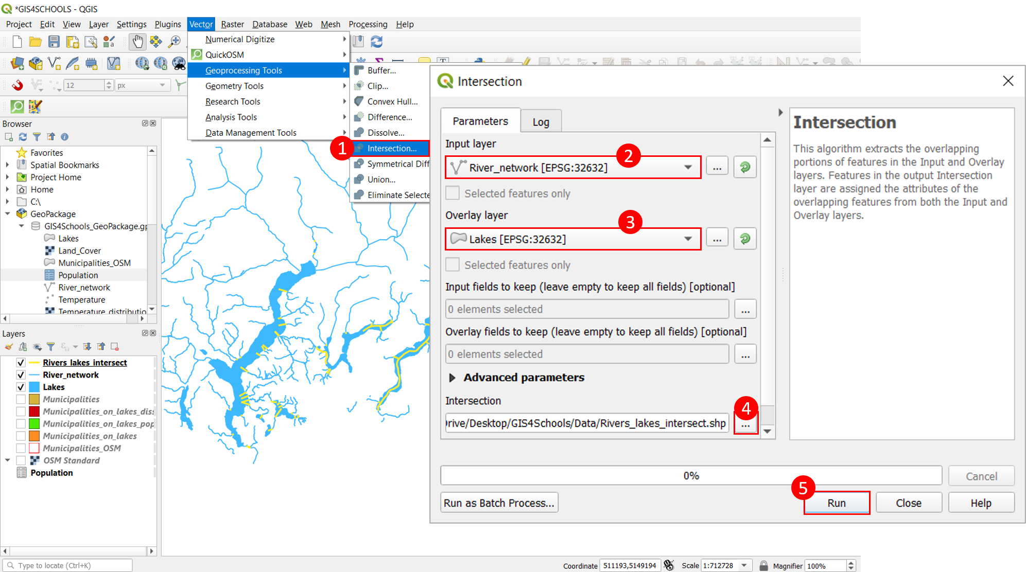
Fig. 2.4.5.1 – Intersection configuration interface. The result of the intersection operation is shown: Rivers_lakes_intersect (yellow lines).

2.4.6. Geoprocessing tools for vector data: buffer

A buffer is the respect area within a fixed distance from a geographic element. It is a very useful tool in proximity analyses. Two types of buffer may be created: a fixed distance buffer and a variable (or dynamic) distance buffer. Let us suppose that we want to create a respect area around the river network. With a first example, we are going to create a fixed-distance buffer, equal for every river segment; afterwards, we are going to create a variable-distance buffer, depending on the river length.

For this purpose, let us first calculate the length of every river network segment with the field calculator. Let us start an editing session: right click on the layer River_network → Toggle editing. Open the attribute table of River_network and click New field. Name the new field Length and assign the Type “Decimal number (real)”. Open field calculator, check the option Update existing field and select Length as the field to be updated. In the Expression tab, search for and double-click Geometry → $length. Finally, click OK and the length of every feature shall be calculated. Save and stop the editing session.

Now we can create a fixed-distance buffer around the river network. Let us suppose to use a distance of 50 m. In the main menu, select Vector → Geoprocessing Tools → Buffer (1). In the configuration interface, select as Input layer River_network (2) and assign 50 meters in the Distance bar (3); check the option Dissolve result (4) and save the buffer area as a new shapefile, specifying an adequate path (clicking the ellipses symbol). Let us name the new shapefile River_network_buffer_fixed (5). Then, click OK (6). Fig. 2.4.6.1 shows the configuration interface for a fixed-distance buffer as well as the resulting layer (in yellow).

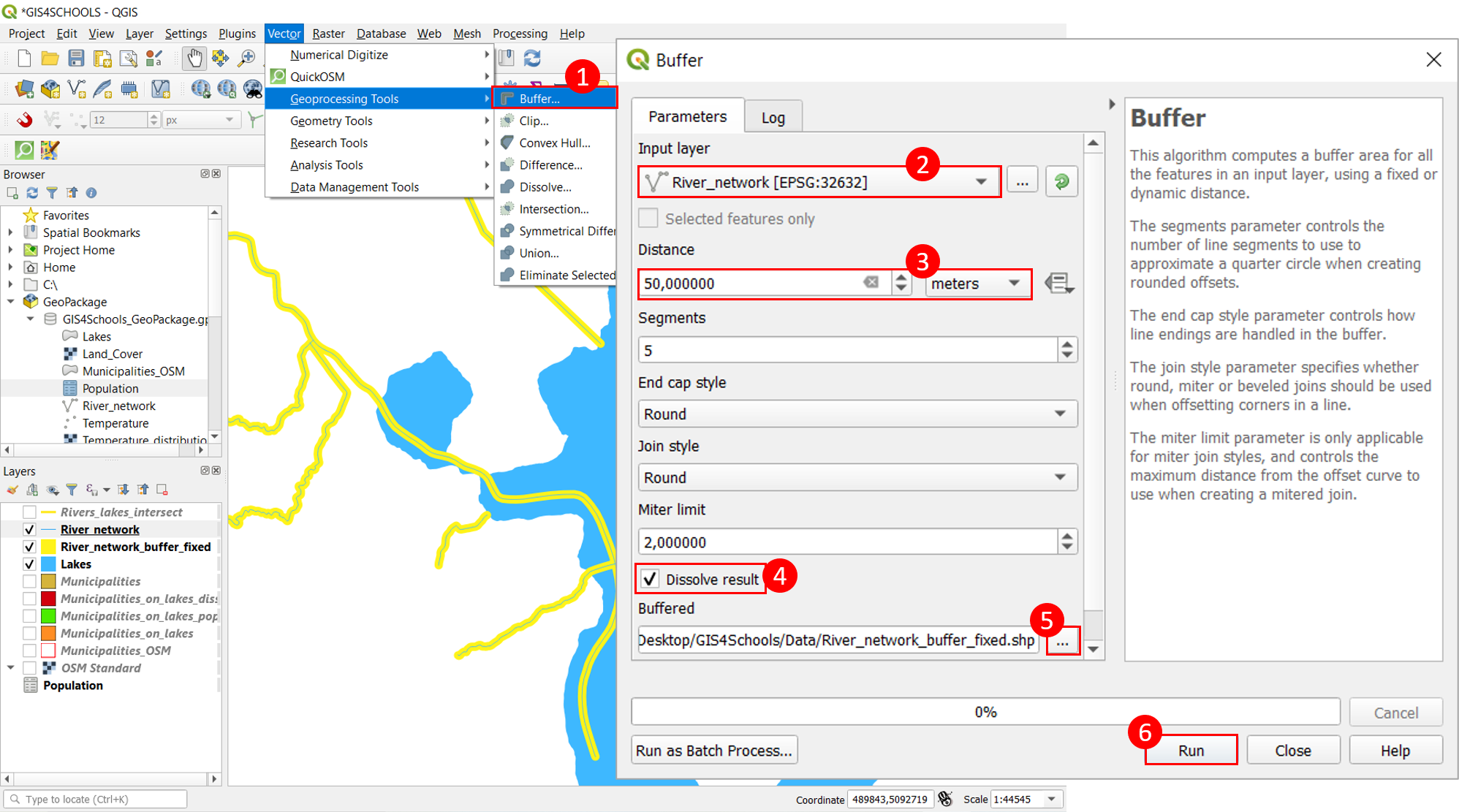
Fig. 2.4.6.1 – Configuration interface to create a fixed-distance buffer.

Now we are going to create a variable-distance buffer around the river network. In particular, the distance will be equal to 50 m for rivers with length higher than 50 km and 20 m for those with length lower than 50 km.

For this purpose, let us add a new field to the shapefile River_network to differentiate between two buffer distances: Toggle editing on the layer River_network, open its attribute table and select New field. Let us call the new field Distance and assign the Type “Whole number (integer)”. Now, let us use the tool Select by Expression that we have previously described, in order to select the river segments with length higher than 50 km: let us write the expression “Length > 50000” and click Select Features. Now that the selection has been applied, open the Field calculator and select Update existing field (choosing the field Distance), write in the expression tab the number 50 and click OK. Then, use the Invert selection tool to select the river segments shorter than 50 km: with the Field calculator, assign the value 20 to the selected features in the field Distance. Finally, deselect all features, save and stop the editing session.

Now we can create the two buffer areas. Let us open the configuration interface: Vector → Geoprocessing Tools → Buffer (1). Select as Input layer River_network (2) and, in the Distance tab, select Data defined override → Field type: int, double, string → Distance (integer) (3). Then, check the tab Dissolve result (4) and name the resulting shapefile River_network_buffer_variable.shp (5), choosing an adequate path (usual folder of the exercise session). Finally, click Run (6). Fig. 2.4.6.2 shows the configuration interface for the variable-distance buffer as well as the resulting layer (in orange).

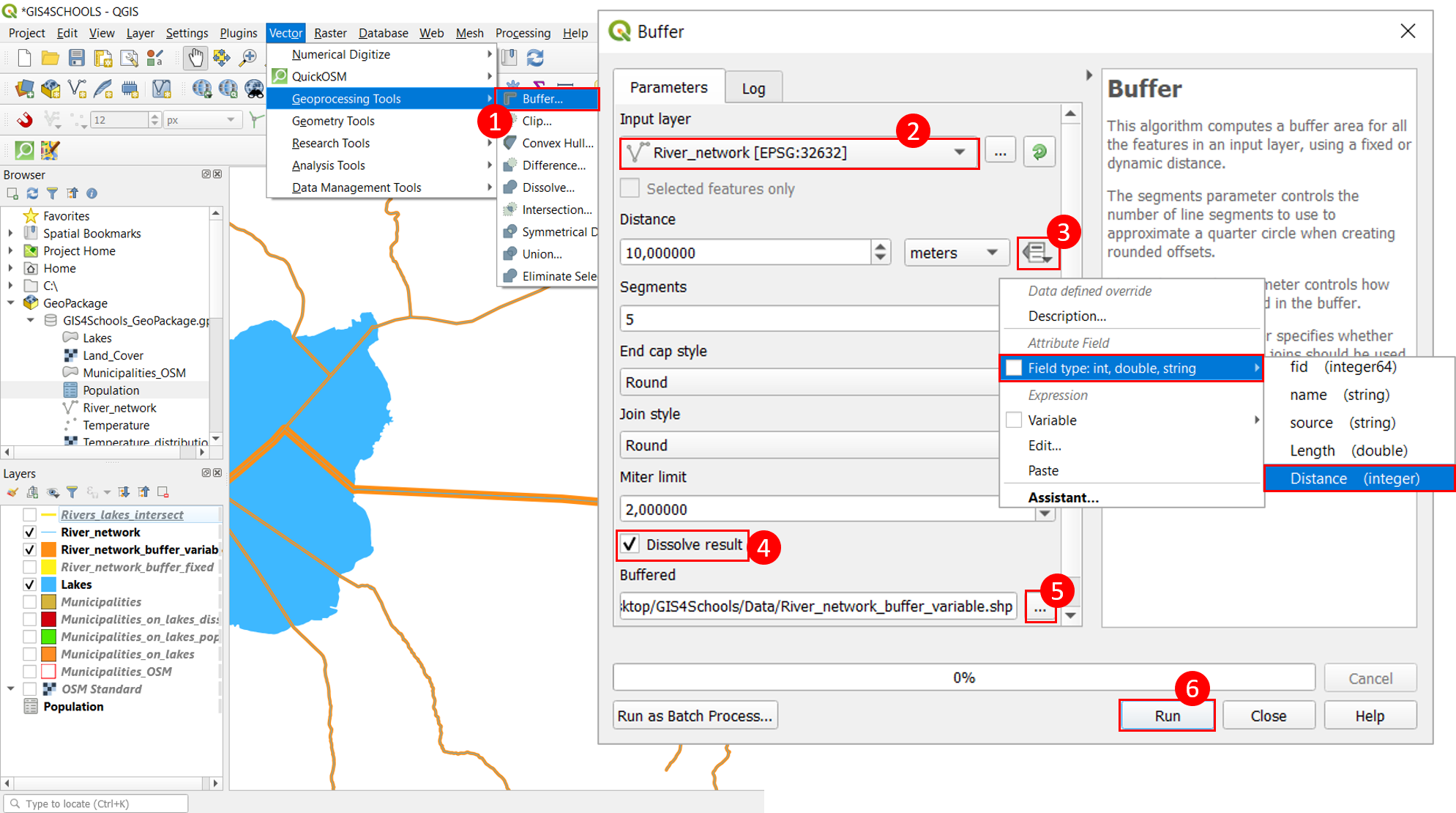
Fig. 2.4.6.2 – Configuration interface to create a variable-distance buffer. The result (buffer area) is shown: River_network_buffer_variable (orange polygon).

2.4.7. Rasterization

In the last part of this exercise session we are going to show how to rasterize a vector file, that is, how to convert a vector layer into a raster layer. The shapefile that we are going to convert is Temperature.shp (corresponding to a layer of points).

In order to convert a vector file to a raster file in QGIS, the tool Rasterize may be used: in the main menu, select Raster → Conversion → Rasterize (Vector to Raster) (1). Select as Input layer Temperature (2); select Value as Field to use for a burn-in value (3) (this option defines the attribute field from which the attributes for the pixels should be chosen). Select Pixels as Output raster size units (4) (this means that the geometric resolution that is going to be defined is expressed in pixels and not in georeferenced units). Specify the value 1000 for both Width/Horizontal resolution and Height/Vertical resolution (5). Choose the adequate raster extent, by clicking on the ellipses symbol in the Output extent space and selecting Use Layer Extent → Temperature (6) (in this way, the resulting raster file will have the same spatial extent as the original vector file). Finally, choose the proper file path and name (7) (for example, Temperature_raster) and click Run (8): the raster will be saved in GeoTIFF format. Fig. 2.4.7.1 shows the configuration interface for the rasterization.

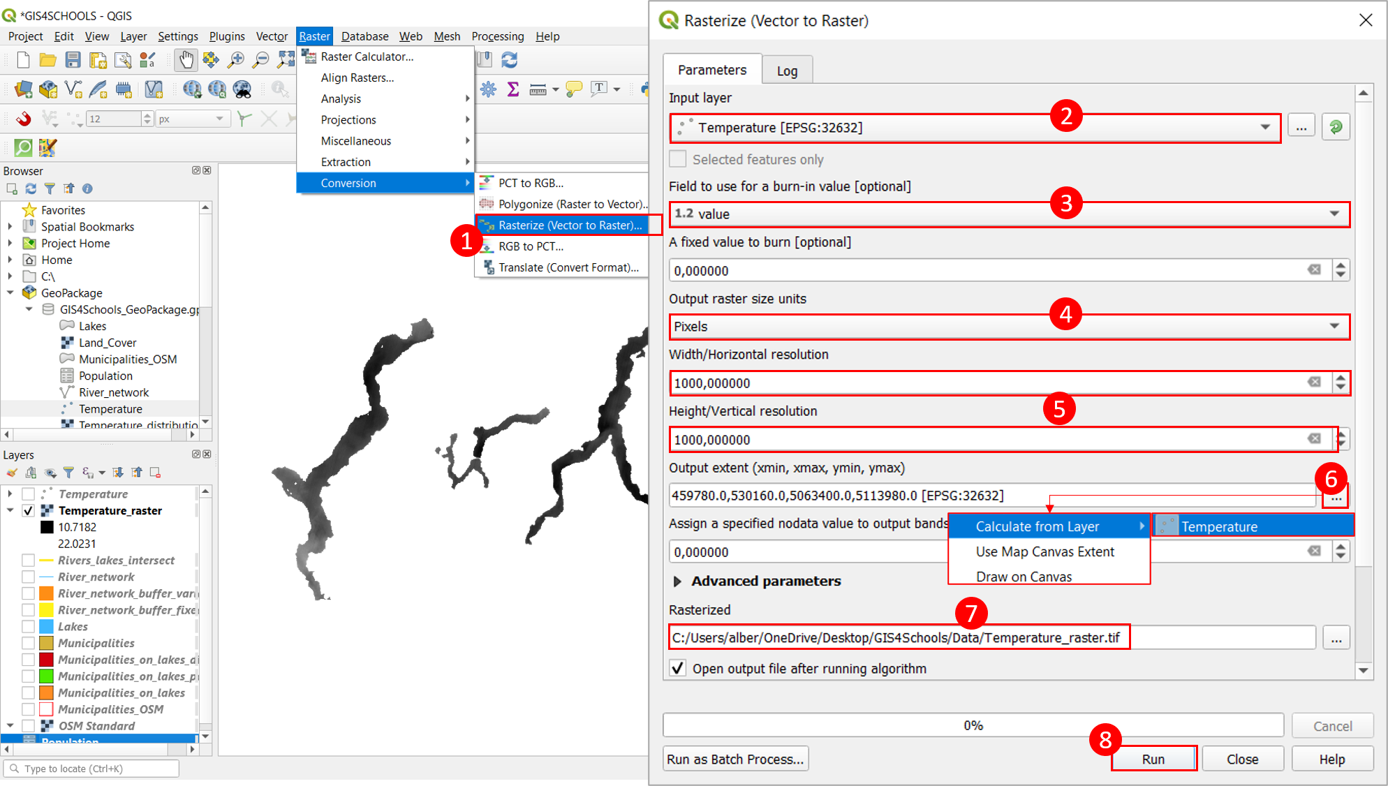
Fig. 2.4.7.1 – Configuration interface for the rasterization process.