1.8. QGIS visualization for vectors
Visualization is probably one of the simplest tasks in GIS, nevertheless, it is important to make geographic data visually informative. This can be achieved by changing visual properties (i.e. styling) geographic data. In this exercise, we will see some basic styling on different types and vector data. Vector styling will be shown on the example of vectors:
Municipalities_OSM: vector of polygons representing municipalities. It has 3 attributes:
- fid – unique feature identifier (number)
- source – information about data provider
- name – names of the different municipalities represented by this vector
River_network: vector of lines representing rivers. It has 3 attributes:
- fid – unique feature identifier (number)
- name – names of the different rivers
- source –information about data provider
Temperature: vector of points representing lake temperature on a regular grid of points. It has 3 attributes:
- fid – unique feature identifier (number)
- value – the numerical value of the temperature in each point (number)
For maximum visibility of layers it is recommended to keep point features at the top of the Layers list, then line features, and at the end to have polygons features as this is the order the layers are displayed in the Map panel (Fig. 1.8.1). We can easily rearrange the order of layers by selecting one of them and dragging and dropping it to the preferred position.
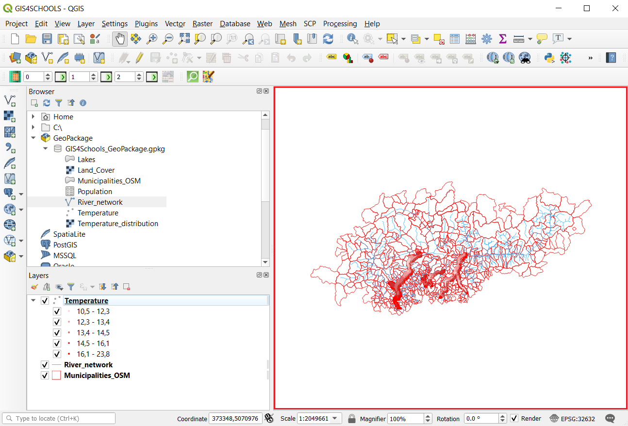
Fig. 1.8.1 – Rearrange layers order
The style for a layer can be set/changed from the layer properties (Fig. 1.8.2). It is necessary to right-click on the layer (1) and click on Properties (2). Then on the Symbology tab (3) we can access different styling options.
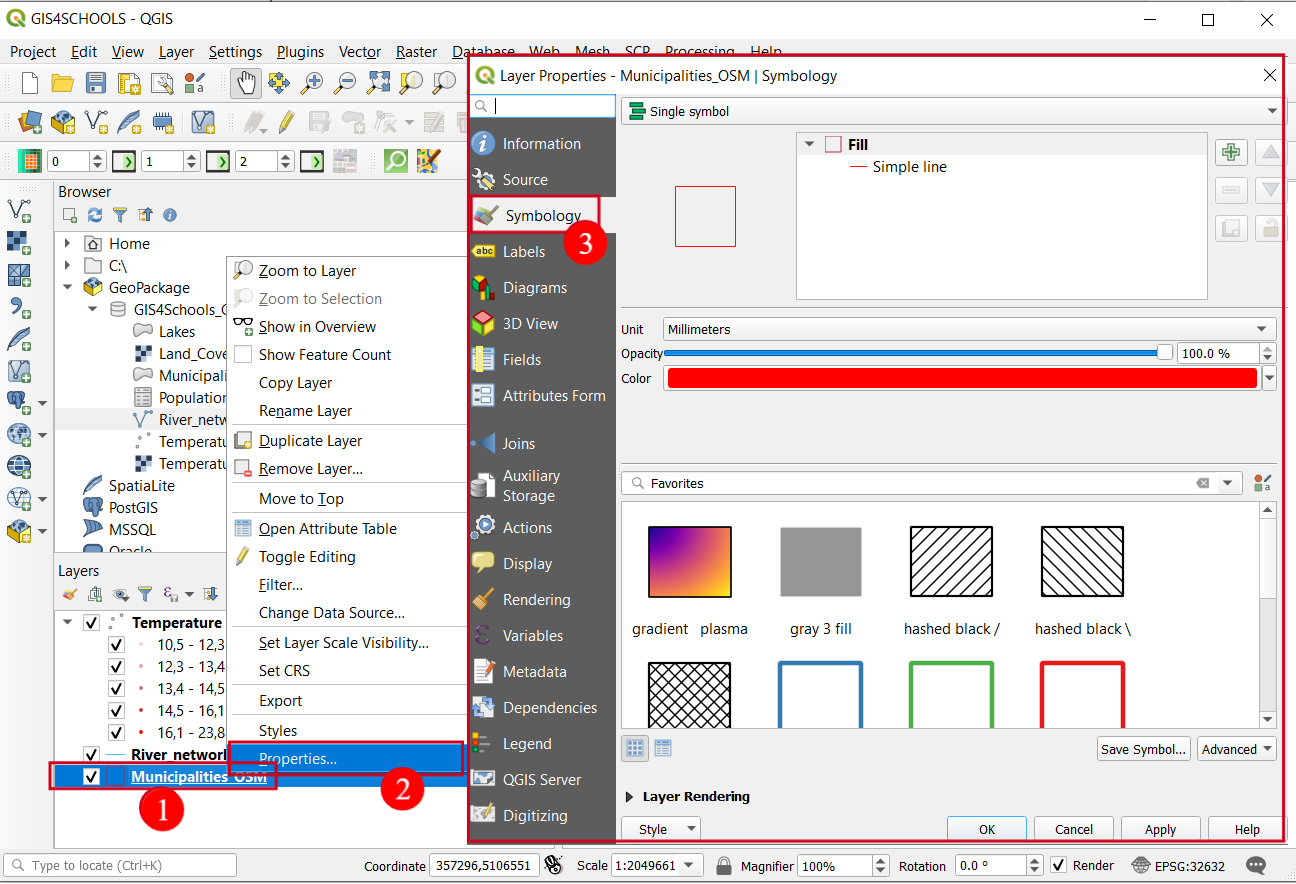
Fig. 1.8.2 – How to modify visualization from layer properties
Alternatively, it is possible to activate Layer Styling Panel (Fig. 1.8.3). It is done from the View menu (1) → Panels (2) by ticking the box next to Layer Styling Panel (3).
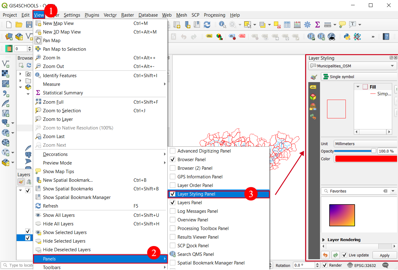
Fig. 1.8.3 – How to modify visualization from Layer Styling Panel
Before we start setting our style for features, let us cover some styling basics. The first thing to be defined in the Symbology tab (1) when styling is concerned is the symbol type. It is done from the drop-down menu (2) (Fig. 1.8.4). Some types of symbols are common for every type of feature - points, lines, and polygons, such as:
- Single Symbol – single symbology for all the features of the vector
- Categorized – splits features into categories according to an attribute
- Graduated – splits features into intervals according to a numerical attribute
- Rule-based – splits features according to the specific rules
However, some types of feature have particular symbols (e.g. Inverted Polygons and 2.5D for polygon features).
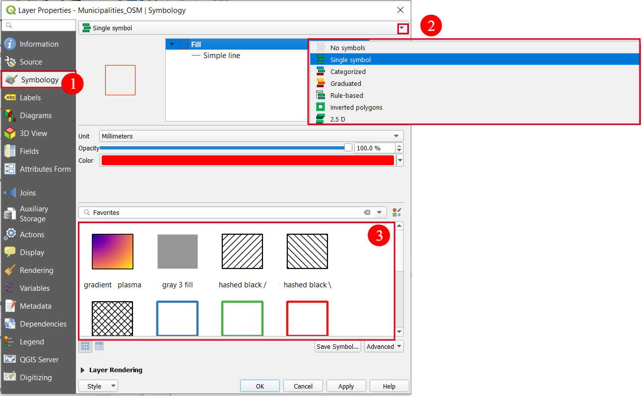
Fig. 1.8.4 – Vector symbols
1.8.1. Single symbol style
In this exercise, regarding the polygons, we are going to set a simple style (Fig. 1.8.1.1). We can set a Single symbol (1) with dark yellow color as fill and black dash-line stroke. To do so select sub-level of Fill (2), and then Simple fill (3) for symbol type. Select dark yellow for Fill color (4), black color for Stroke color (5), and dash line for Stroke style (6). Click on OK or Apply to apply the style (7).
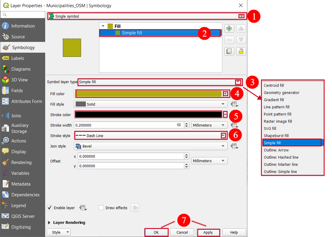
Fig. 1.8.1.1 – Apply simple style based on a single symbol on polygons
To be able to properly see the style applied to the vector of polygons deactivate other layers in the Layers panel (1) as shown in Fig. 1.8.1.2.
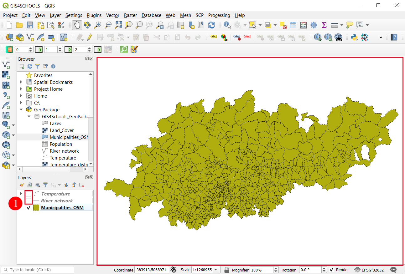
Fig. 1.8.1.2 – The outcome of polygon styling with single symbol simple style
1.8.2. Categorized style
Moving forward, we will set a style for visualizing River_network which is a line feature (Fig. 1.8.2.1). As for the polygons, style is set from the layer Properties on the Symbology tab. In this case, we will see how to group features into categories by using Categorized symbol types. Categorized (1) symbol type is used when there is an attribute whose values can be grouped/categorized. In the case of River_network, there is the attribute source which contains information about the data provider. Select source attribute for the Value field (2) and select a Color ramp (3) (e.g. Viridis) Finally, click on Classify (4) to make the classification. Categories will be previewed in the central part of the window (5). Click on OK or Apply (6) for changes to take place.
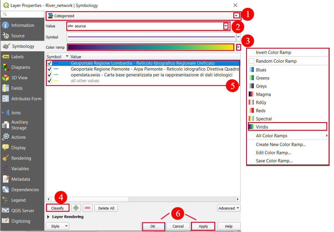
Fig. 1.8.2.1 – Apply Categorized style on lines
In Fig. 1.8.2.2 we can see the effect of the style applied to lines. Also, we can see categories in the Layers panel if we expand the layer tree.
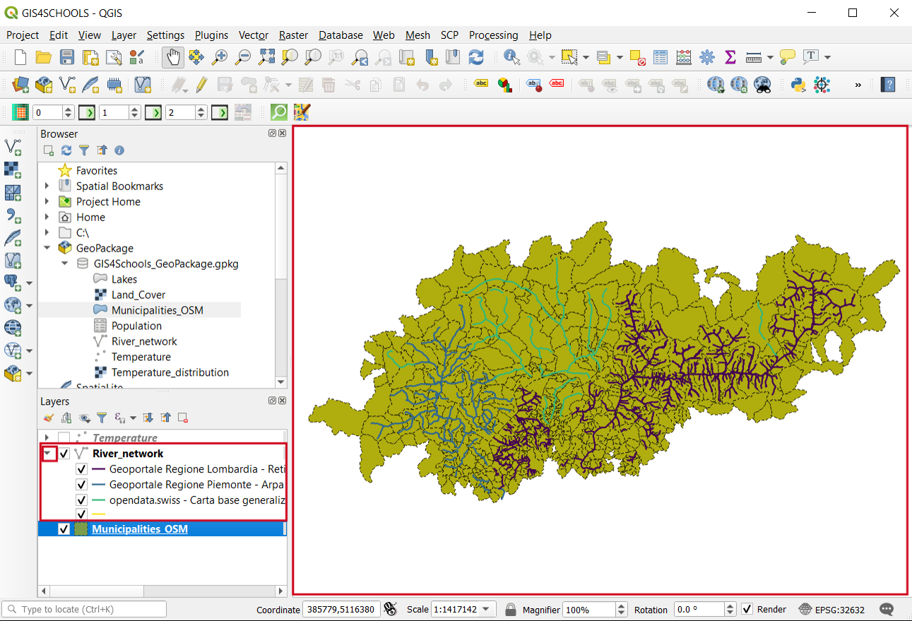
Fig. 1.8.2.2 – The outcome of line styling with categorized style
1.8.3. Feature labels
Another important aspect of vector styling is the possibility of adding labels to the features. It is done from the layer Properties on the tab Labels (1) (Fig. 1.8.3.1). There are different methods for labeling (2). In this exercise, we will focus on single labels. In case of single labels there is one label for each of the features. Labels can be stored as an attribute in the attribute table or they can be defined through an expression. We can display this attribute name as a label by selecting this field for the Value field (3). There are different options for formatting and configuring interaction with labels. We can modify them by selecting the appropriate tab (4). In this example, we only set the Buffer (6) to be drawn (7) because it enhances label visibility. Other options were kept as a default. In the Text Sample (4) field we can see the preview of the text formatting.
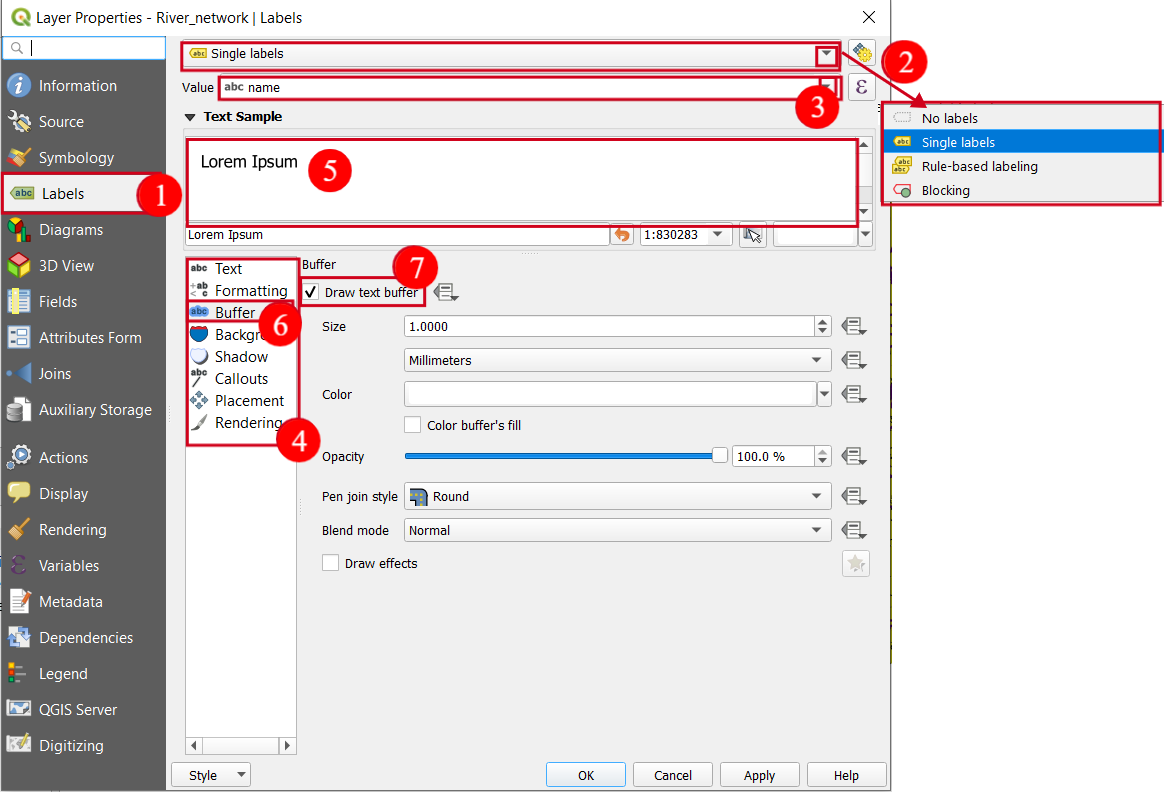
Fig. 1.8.3.1 – Adding labels to the line features
As a result, we have names of some rivers displayed (Fig. 1.8.3.2). We can see that labels have a white buffer around letters.

Fig. 1.8.3.2 – The outcome of line feature labeling
1.8.4. Graduated style
Finally, we are going to set a style for the points layer Temperature ( Fig. 1.8.4.1.). Since there are many temperature records and there are numerical values it is convenient to split them into a certain number of intervals. To do so, the first thing is to set symbol type Graduated (1) which allows making intervals out of the full range of numerical records. Afterward, we select the attribute which contains numerical values (e.g. value) (2). Select Color ramp according to the preferences (3). In this example RdYlBu color ramp is selected (red to blue), so we will Invert Color Ramp (4) to have typical temperature representation – blue to red. Select the mode Equal interval (5) to split values into equal size classes. Then specify number of Classes (6) (e.g. 5) and click on Classify (7). The resulting intervals will be displayed in the preview (8). Click on OK or Apply (9).
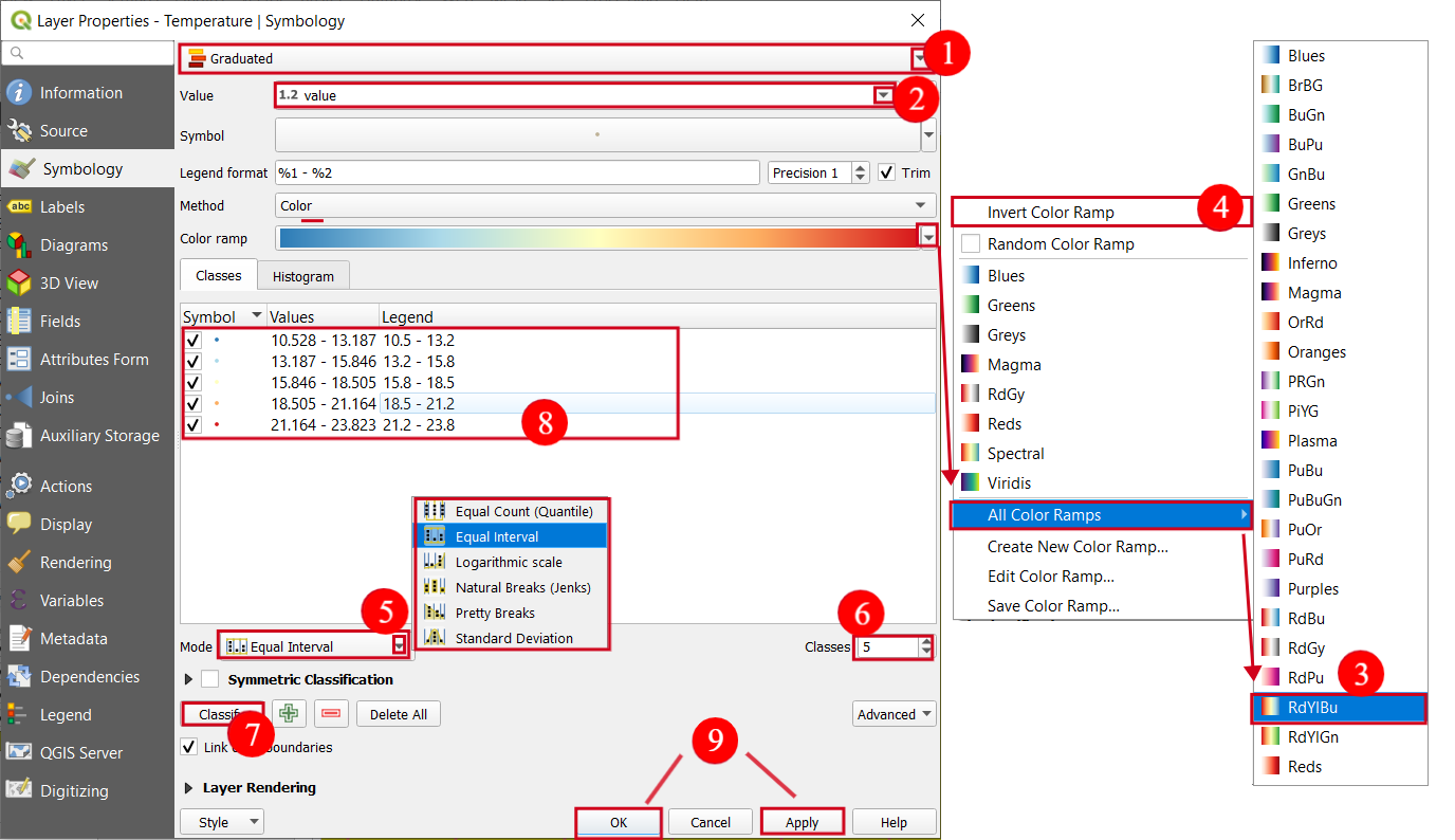
Fig. 1.8.4.1 – Apply Graduated style to the points
To better observe outcomes of the Temperature styling, we will zoom to the extent of the Temperature layer (Fig. 1.8.4.2) by right-clicking on the layer and selecting Zoom to layer (1).
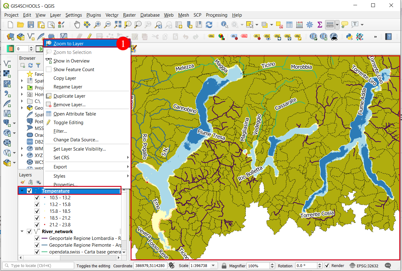
Fig. 1.8.4.2 – The outcome of point styling with Graduated style
1.8.5. Saving and loading style
Style can be saved from the Symbology tab of the layer Properties. Click on Style menu (1) → Select Save style (2). Select one of the three Save styles (3) available (Fig. 1.8.5.1):
- QGIS QML style file
- SLD style file
- Database (GeoPackage)
Let us first check options of the Database (GeoPackage) (3) save the style. Insert a Style name (4) and click on OK (5). The style is automatically saved in the GeoPackage together with a layer and it will be displayed next time River_network is loaded.
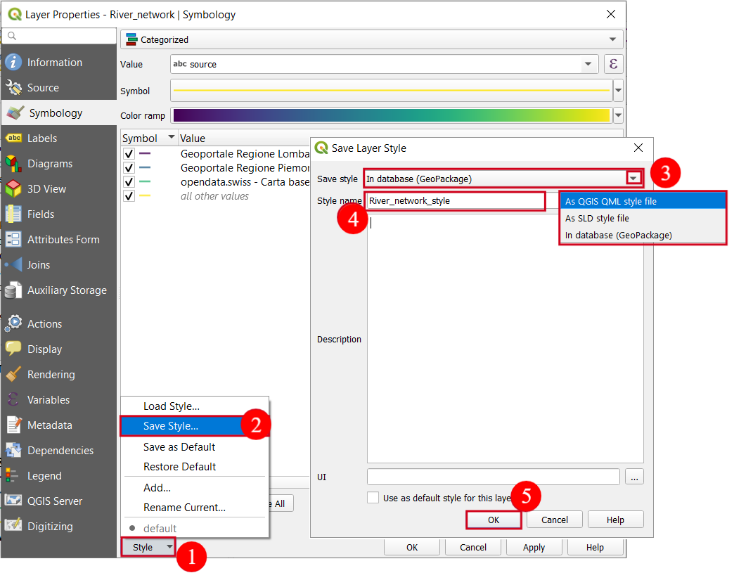
Fig. 1.8.5.1 – Save vector style in the database (GeoPackage)
The other two Save style options - QML and SLD - create a separate style files (Fig. 1.8.5.2). QML (1) is an XML format suited to store styles that QGIS can support. To save a style in this format it is necessary to specify the File path and name (2). It is the only style that allows selecting specific Categories of style to be saved (3). SLD (4) (Styled Layer Descriptor) is an XML schema for the styling map layers. It is not suited only for QGIS, but also for other GIS softwares. To save style as SLD file, specify File path and name (5).
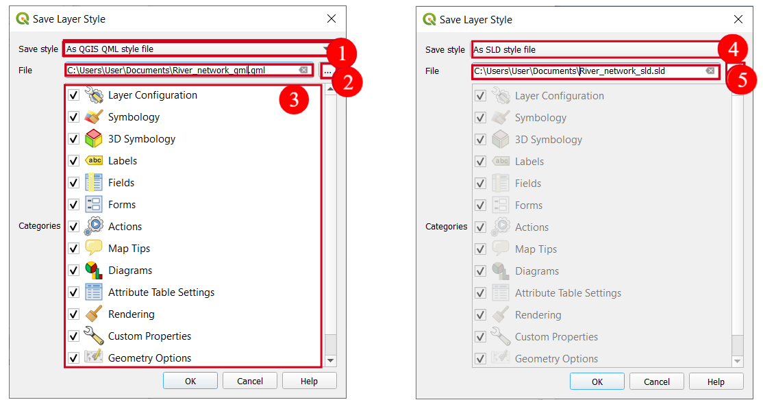
Fig. 1.8.5.2 – Save vector style as QML file (left) or SLD file (right)
In a similar manner to the style saving, an already saved style can be loaded (Fig. 1.8.5.3). Style is loaded from Style menu (1) on a Symbology tab of layer Properties. To load a style saved in a GeoPackage (or other database formats) select Load style (2) → From database (GeoPackage) (3). To load a style from a QML or SLD file select Load style (2) → from file (4). When the style is loaded from GeoPackage we can select some of the styles that were previously saved for this specific layer (5) or some of the previously saved styles of other layers saved in the same GeoPackage (6). Furthermore, we can select style Categories to be loaded (7). To load styles from file, specify the path to the QML or SLD file (8). With QML file we can also select which style Categories to load (9).
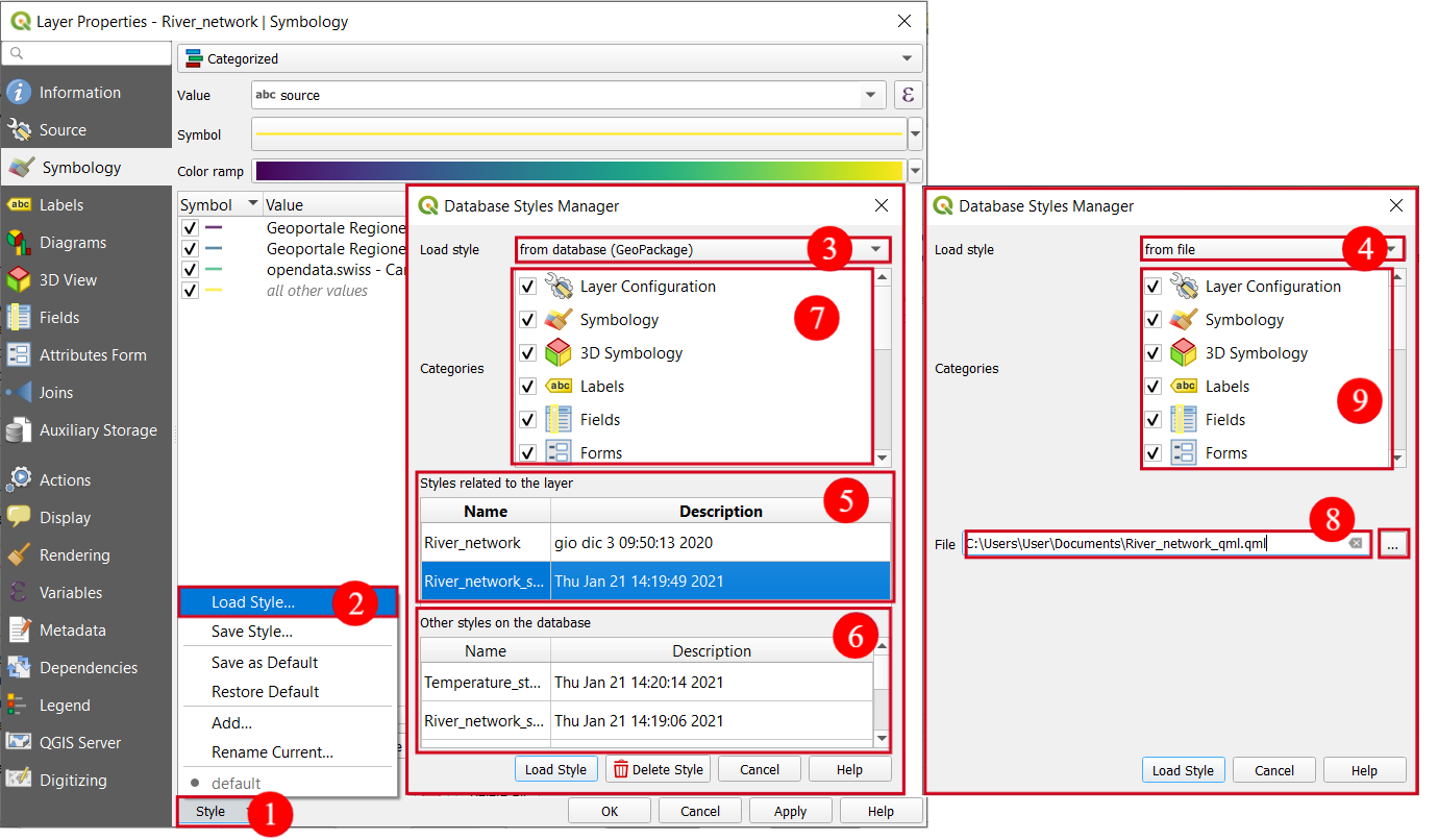
Fig. 1.8.5.3 – Load a style from database (GeoPackage) or from a file
Besides saving a style independently, we can save a QGIS project (Fig. 1.8.5.4) which saves currently loaded layers, their styles, map extents, and settings. QGIS project can be saved by selecting menu Project (1) → Save (2). Similarly, we can resume work on a saved project by selecting Project (1) → Open (3).
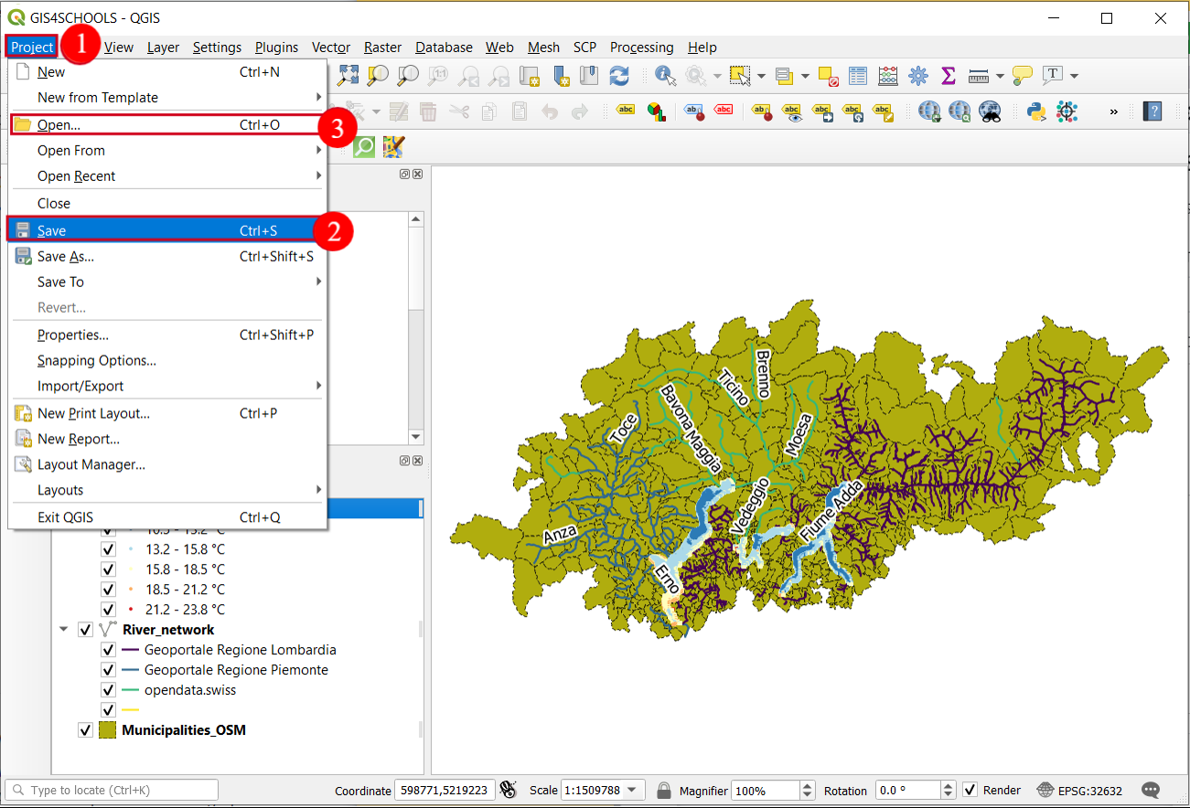
Fig. 1.8.5.4 – Save QGIS project
In this exercise, we have seen different ways of visualizing vector layers. Keep in mind that even if a style in these examples was applied on one type of data (e.g. vector points) it can be applied to other types of data (e.g. lines and polygons). It is also important to mention that the visualization style highly depends on the information we want to expose, but to some extent, it is also a matter of creativity so do not be afraid to experiment with it.