1.11. Atlases
Now that you have seen the importance of both styling and map layout, Atlases can be introduced. The purpose of Atlases is to create many maps with the same template in an automatic way, saving a considerable amount of time in respect to a manual operation. QGIS Atlas allows you to create multiple maps using the records of a vector layer. After selecting a map layer as your index (coverage) layer, a page corresponding to each of its features is generated. QGIS Atlas dynamically adapts the content of the different layout items to each feature in the index layer.
The following layers resulting from the previous steps will be now used to illustrate how to construct an Atlas:
- Municipalities.gkpg (polygons representing the boundaries of the municipalities, including the Province and the Population attributes);
- River_network.shp (lines representing the river network across the lakes basins);
- Temperature_raster (raster representing the lakes surface water temperature).
To start, add both Vector and Raster layers (Fig. 1.11.1, 1) to your project. Before creating a new Layout, select the Temperature_raster in the Layers Panel (2) to modify its symbology. Instead of opening the layers properties, we can also right-click on one of the upper toolbars and flag the box of the Layer Styling Panel (3) to visualize it on the right. From here you can modify the symbology of every layer while looking at the map. Select the Singleband Pseudocolor representation from the drop-down menu (4) and modify the threshold values (10.75; 13.5; 16.5; 19.25; 22) to have a simpler and shorter legend later (5). Select then the River_Network layer and set its symbology as in the example (light blue continuous line of 1mm width). Click then on the New Print Layout icon (6) to open the Create print layout Title window (7). Define a title (“Atlas” in this the example) and press OK (8).
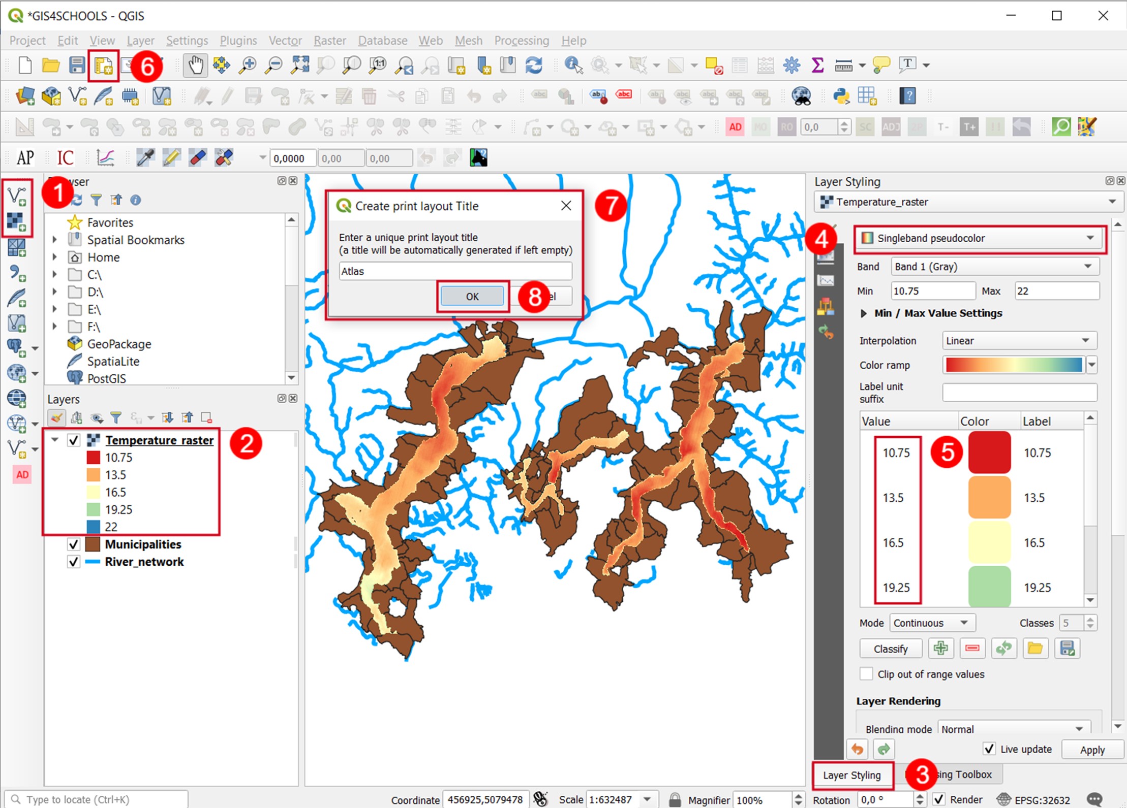
Fig. 1.11.1 – Add layers, change symbology and create a new layout
A new window with the Layout interface will open (Fig. 1.11.2). Before approaching the Atlas logic, click on View (1) and then on Show Grid and Snap to Grid (2) to visualize a background grid and activate the snaps to its nodes. This will facilitate the creation of new items with appropriate spacing and alignments. In the Items column, click on the Atlas section among the four available (3). After flagging Generate an Atlas (4) the Configuration and Output sub-sections will become editable and the Atlas Preview icon (5) visible. Select the Municipalities layer as Coverage layer (6) and its attribute name as Page name (7). Please note that the coverage layer can only be a vector.
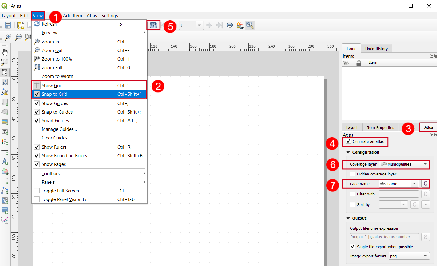
Fig. 1.11.2 – Grid view and snap, Atlas creation and settings
Refer to Fig. 1.11.3 steps and result. Right clicking on a point on the white canvas (1) and select Page Properties (2). In the Item Properties section (3) you have the possibility of changing page Size and Orientation (4), choosing among international formats, or defining customized measures. For this exercise, select an A3 Landscape page. After that, add to the layout all the items that you have seen in section 1.9 (map, title, legend, scale bar and north arrow) as shown in the example.
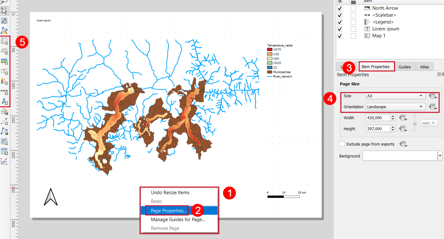
Fig. 1.11.3 – Add items to layout and set page size
Now that the elements are in place it’s time to modify their properties to let the atlas control their content. Click on the white arrow in the left Toolbox to enter the Select/Move item mode (Fig. 1.11.4, 1) and then click on the map (2). In the Item properties section, you are now able to change all the settings of the selected item. For the Map item, flag the Controlled by Atlas checkbox (3) and select the first visualization option among the three available below (4). In this way, the map of every single page will be centered on the corresponding feature of the coverage layer (Municipalities), leaving a margin corresponding to the 25% of the image from the map frame, that can be activated by flagging the Frame checkbox (5).
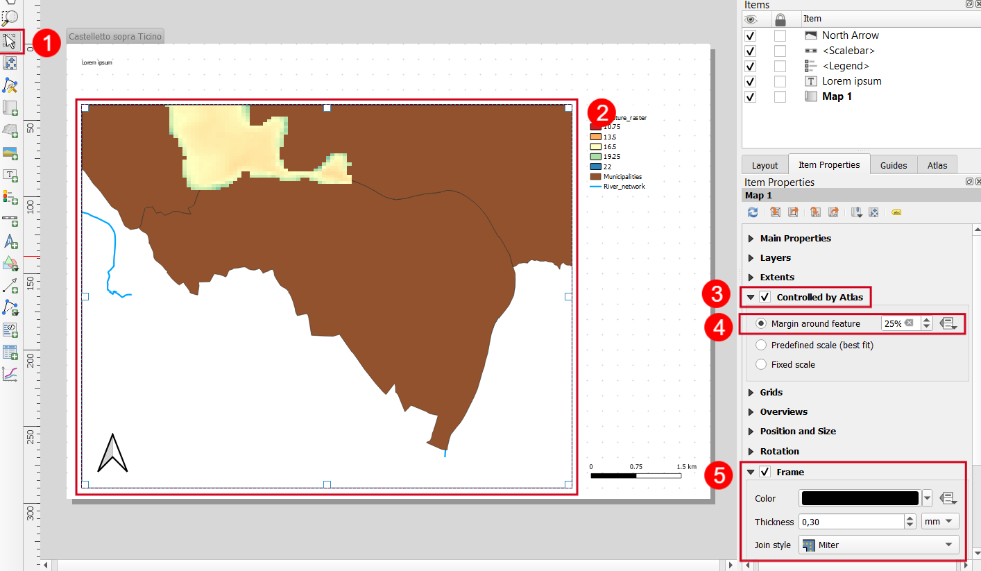
Fig. 1.11.4 – Atlas control on map item through item properties
We proceed with the Title (Fig. 1.11.5). As done before, select the title item on the map and look at the Item properties section. The default content is the Lorem ipsum text that has to be deleted. To make a dynamic title, adapting to the map content, we need to define it as an expression (2). Open the Insert Expression window (3), type in the expression space the following one (4) and press OK (5):
concat("name", ' (', "province", ')')
This expression literally means to write the Municipality name followed by the corresponding province between brackets. The “…” identify the field of a layer while the ‘…’ identify text strings. Finally go in the Appearance section and increase Font size up to 30 points (6).
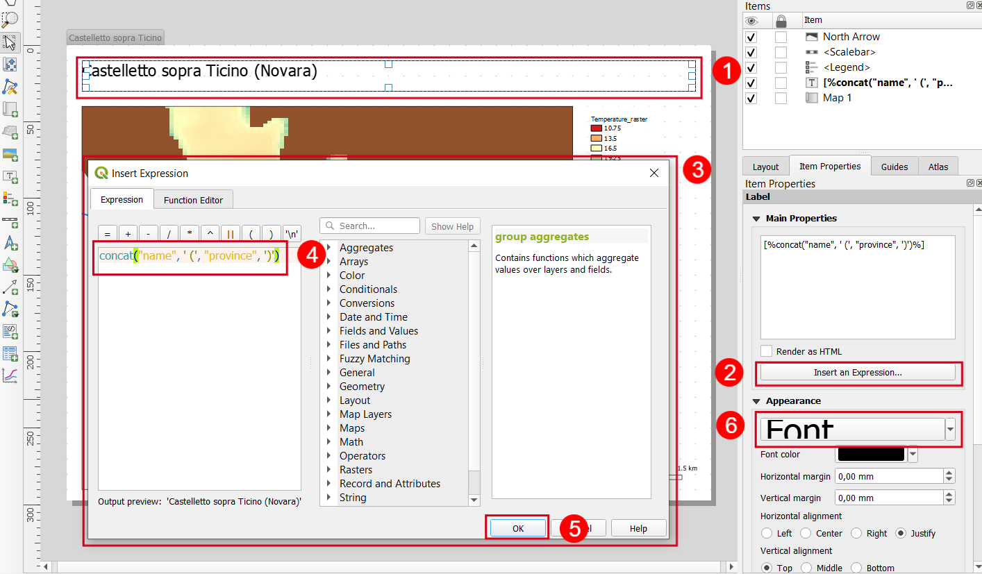
Fig. 1.11.5 – Atlas title driven by inserting an expression in its item properties
Fig 1.10.5 – Atlas title driven by inserting an expression in its item properties The other elements don’t need particular settings except for some graphical preferences that can be defined later. Now the Atlas is properly set but the symbology of the layers is still independent of it. We now want to set a different symbology for the active feature of the Municipalities layer in respect to the other features of the same layer. Leave the Layout window and go back to the main QGIS one. Select the Municipalities layer in the Layer Panel (1) and in the Layer Styling Panel select a Rule-Based Symbology (see Fig. 1.11.7, 1). Add a new rule by clicking on the green + symbol (2) and double click on the record that appears (3) to enter the Edit Rule mode. You can now define a Label (Fig. 1.11.6, 2, Active) and a criterion through an expression (3) for this rule. Click on the ε symbol to open the Expression String Builder window and type the following one (4):
$id = @atlas_featureid
In this way, the active atlas feature has been separated from the others and a dedicated symbology can be now defined in the Symbol section. Set Fill style as no brush, Stroke colour as red and Stroke width as 2mm (5) and click on Apply (6). On the map, you can now see a preview of the symbology for the active feature (7).
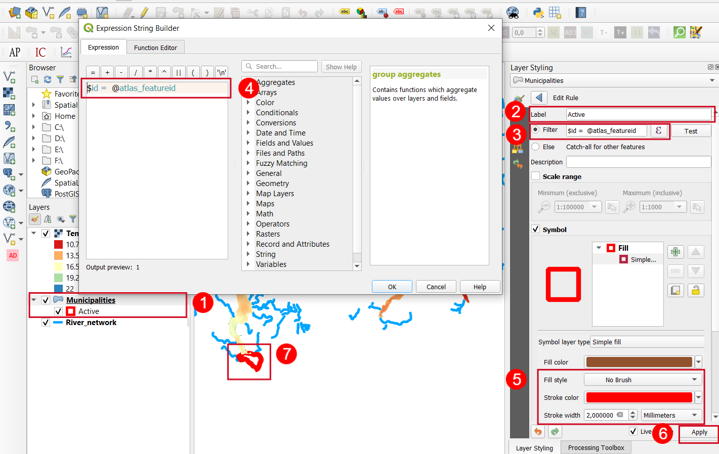
Fig. 1.11.6 – Rule-based symbology for vector layer, identifying atlas active feature
Refer to Fig. 1.11.7 steps and results. Repeat the same operation to set another symbology for the remaining features. In this case, the expression will be:
$id is not @atlas_featureid
The symbology will be instead a solid white Fill with 80% opacity, to be set directly in the color definition, with a black continuous stroke of 0.5mm of width. As now we have different symbologies within the same layer, we may need to define which of the two should be represented first. Click on Symbol Levels (4) and type 1 for the active layer, leaving 0 for the other. In this way, the active layer will be drawn later, going so on the top of the others (5).
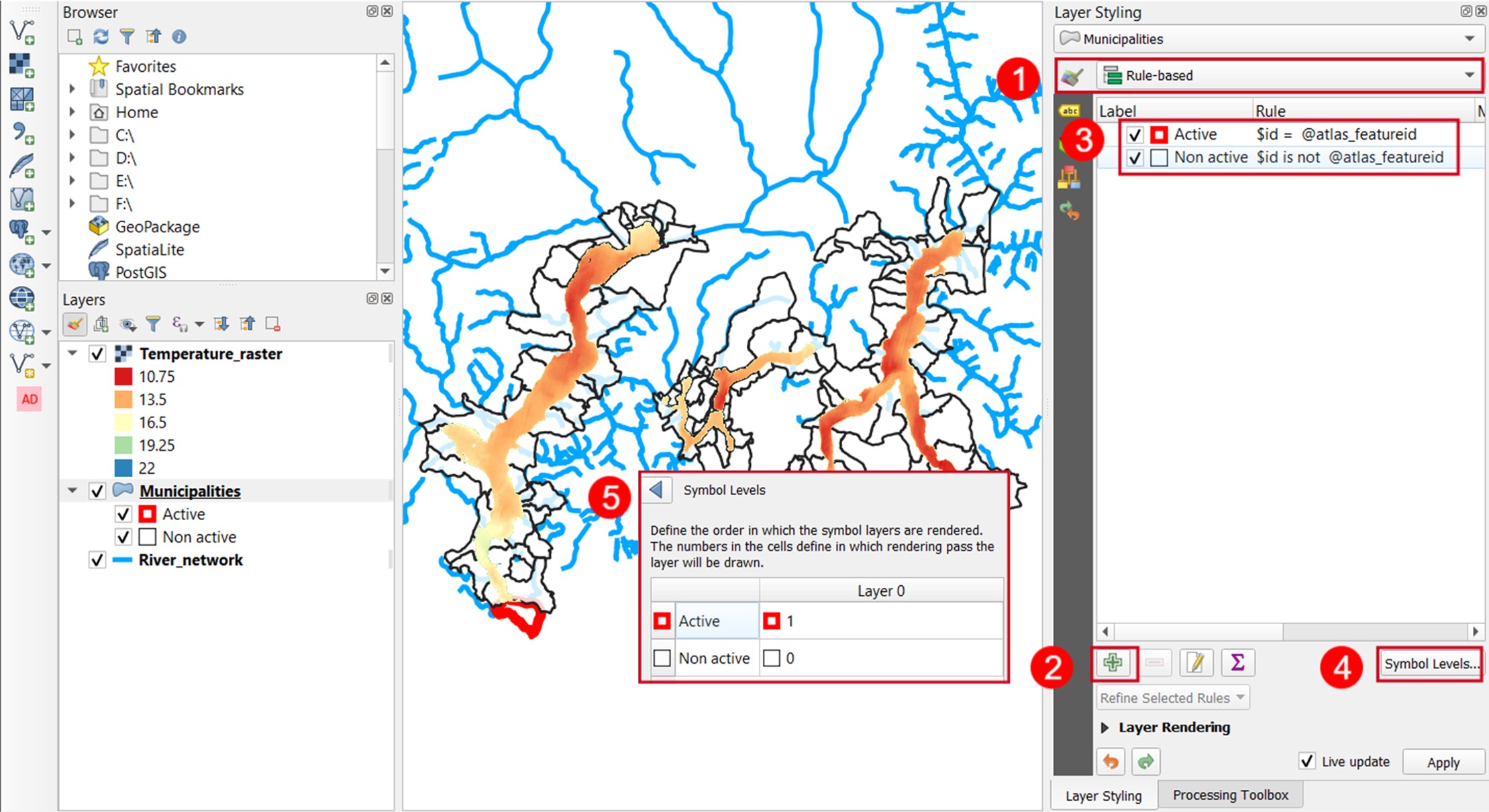
Fig. 1.11.7 – Rule-based symbology, symbol levels definition for visualisation priority
The same logic can be applied to the visualisation of Labels. In Fig. 1.11.8 is shown how to insert a Description (1, Pop ), a Filter or criterion for the rule (2, expression [2] ) and in the Labels section, the content of the label with a Value (3) choosing the population attribute from the drop-down menu. In the Text section (4) modify the Size setting it to 20 points and in the Background section (5) flag the Draw Background checkbox (6) and define the Size on X and Y direction for the buffer (7, 2mm ). In this way, a rectangular white box slightly exceeding the label text will be generated, as visible on the map (8). Before going back to the Layout, we can add a background map. Click on the XYZ Tiles in the Browser panel and right-click on OpenStreetMap (9) to Add the layer to the project. It will appear both on the map and on the Layer Panel (10) where it has to be moved at the bottom of the list. Finally, move the Municipalities layer at the top of the list, above Temperature_raster.
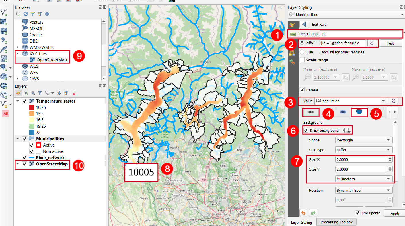
Fig. 1.11.8 – Rule-based label and add OpenStreetMap as background
To conclude the exercise, go back to the Layout and define the properties of the remaining items starting from the Legend (Fig. 1.11.9 a). Select it (1), add Legend as Title (2) and set its Size to 24 (3), the sub-headings one to 18 (4) and the item one to 14.
Similarly, select the Scale bar (1) and modify its style to Line Ticks Up (2) and increase its Font size to 14 points (Fig. 1.11.9 b).
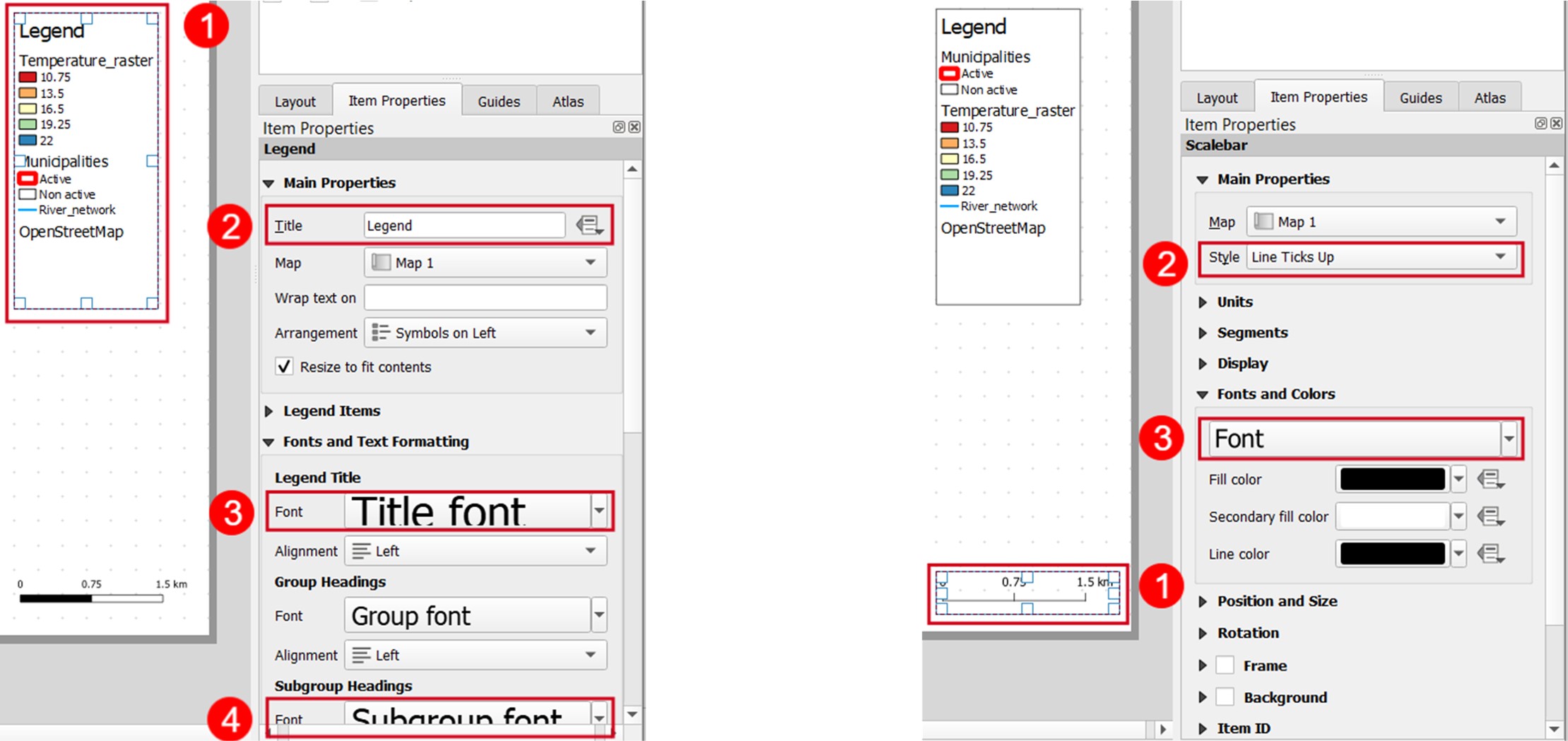
Fig. 1.11.9 – a) Legend properties edit; b) Scale bar properties edit
The Atlas is finally complete. To start navigating its pages click on the Preview Atlas icon (Fig. 1.11.10, 1) and use the arrows (2) to move one or all steps backward or forward. Alternatively you can directly select from the drop-down menu (3) the specific page that you are looking for. This result can be easily exported as .pdf, .svg and .jpg clicking on the Export Atlas icon on the right (4).
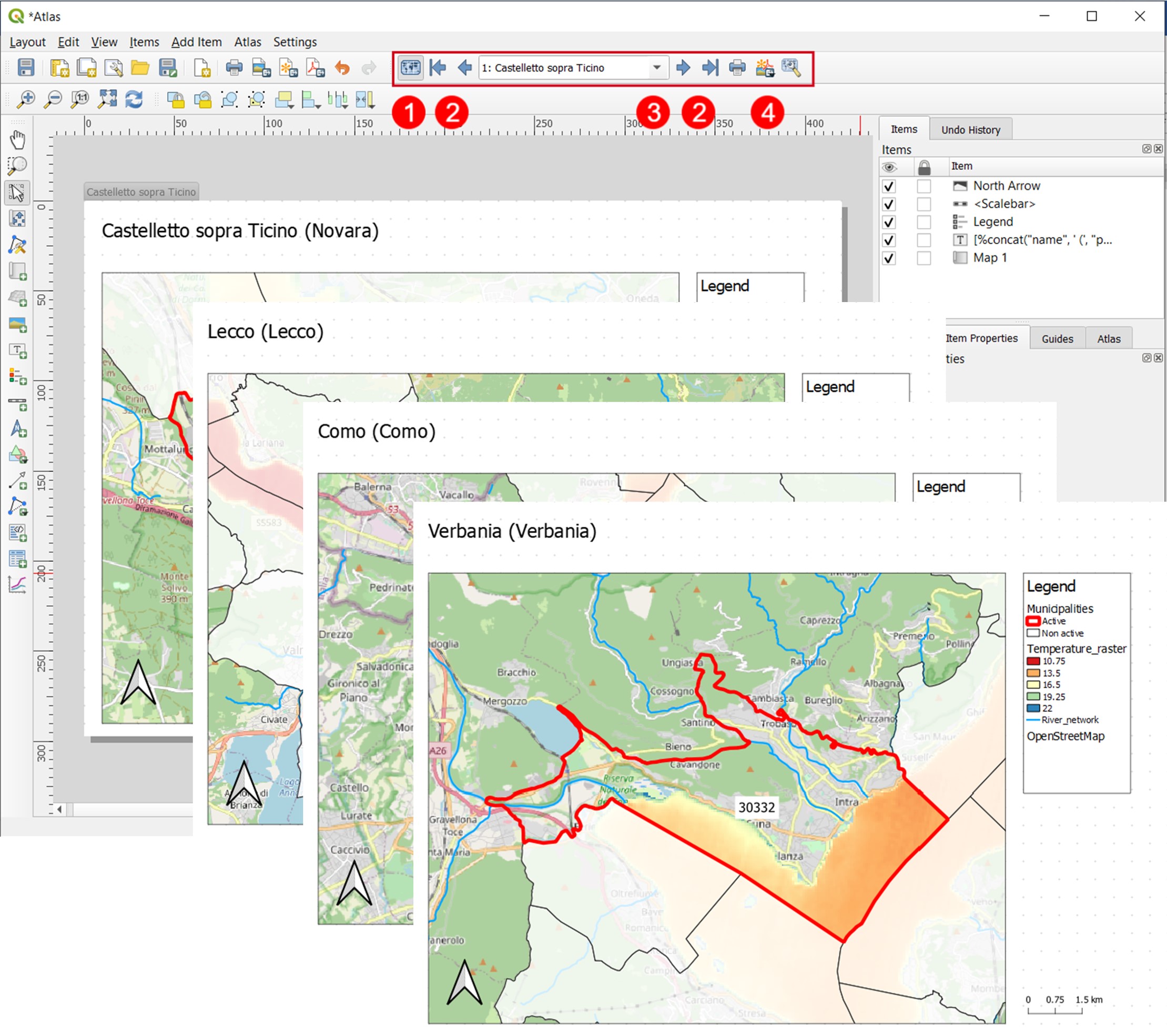
Fig. 1.11.10 – Atlas preview, navigation through pages and output generation
References: