2.2. Accessing OGC services with QGIS
QGIS allows the connection to servers offering geospatial data in compliant with the OGC service standards.
Open QGIS and, in order to have some contextualisation data, upload the geopackage that was used for the previous course, zooming to the extension of the layer (Part 1).
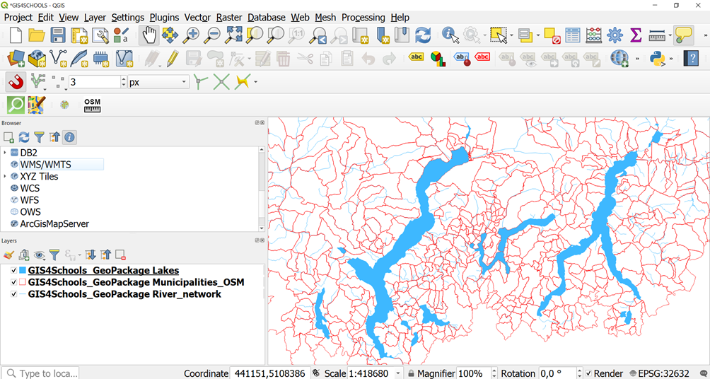
Fig. 2.2.1 – Visualisation of the GIS4Schools Geopackage
To import a layer using OGC services, click on menu Layer → Add Layer and then select the specific layer you are interested in. The following options are available:
- Add WMS/WMTS
- Add WCS
- Add WFS
In the following we will see how to connect to these services.
2.2.1. WMS/WMTS
To add an OGC WMS layer, click on menu Layer (1) → Add Layer (2) → Add WMS/WMTS Layer (3) (Fig. 2.2.1.1). A new window appears. Click on the New button (4) for creating a new service connection.
The first two layers we want to add are EFAS landslide susceptibility and EFAS observed precipitation available in the Joint Research Centre Data Catalogue.
The former [1] presents the spatial likelihood of landslide occurrence in 5 classes as a 1 km raster data set and represents the risk of landslides at a given location, particularly when flash floods are forecasted.
The latter [2] shows the accumulated amount of precipitation for the current day [in mm] with a horizontal resolution of 5 km.
The service, which we will name EFAS, is a WMS-T, a Web Map Service Time, because the available data varies day by day. The access URL is https://www.efas.eu/api/wms/?request=getcapabilities. Once inserted the Name (5) and the URL (6), we can click OK (7) to connect to the service and see which data layers are available.
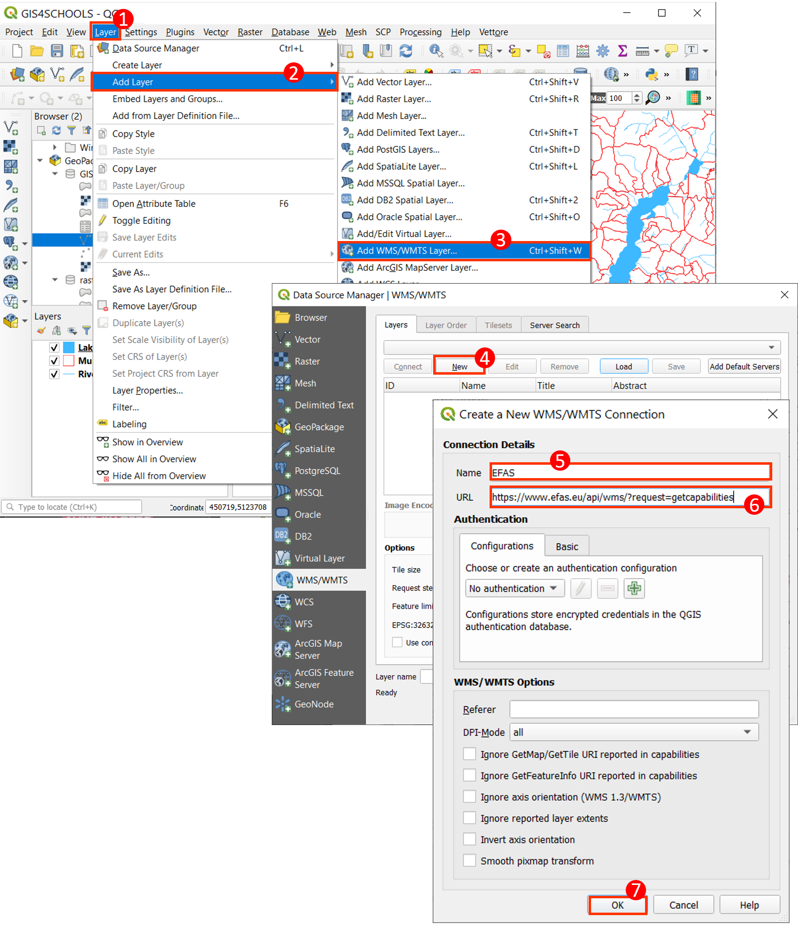
Fig. 2.2.1.1 – Create a connection to WMS services with QGIS
We click the Connect button (1) and, scrolling the list, we select before the Landslide Susceptibility (2) and then the Observed Precipitation (3) services; once the service is selected, we click Add (4) (Fig. 2.2.1.2).
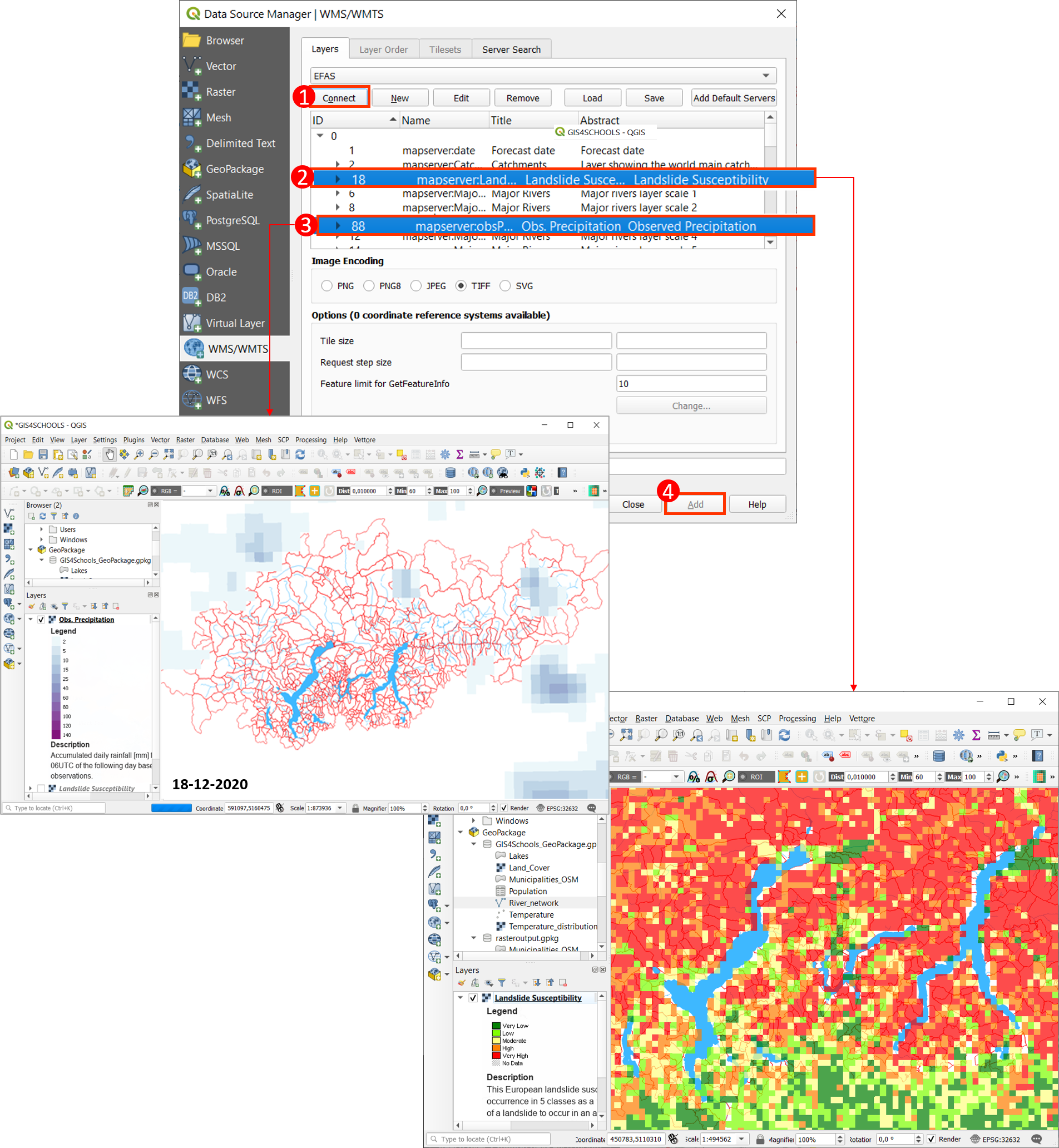
Fig. 2.2.1.2 – Connecting to the WMS services Landslide Susceptibility and Observed Precipitation
As the last step of the WMS section, let us examine where we find the pieces of information related to the XML file which is replied by the server when the client sends a GetCapability request. For that step, carefully compare the EFAS Services GetCapability XML related to the Susceptibility Map with what you find right clicking on the layer (1) and selecting Properties (2) → Information (3) (Fig. 2.2.1.3).
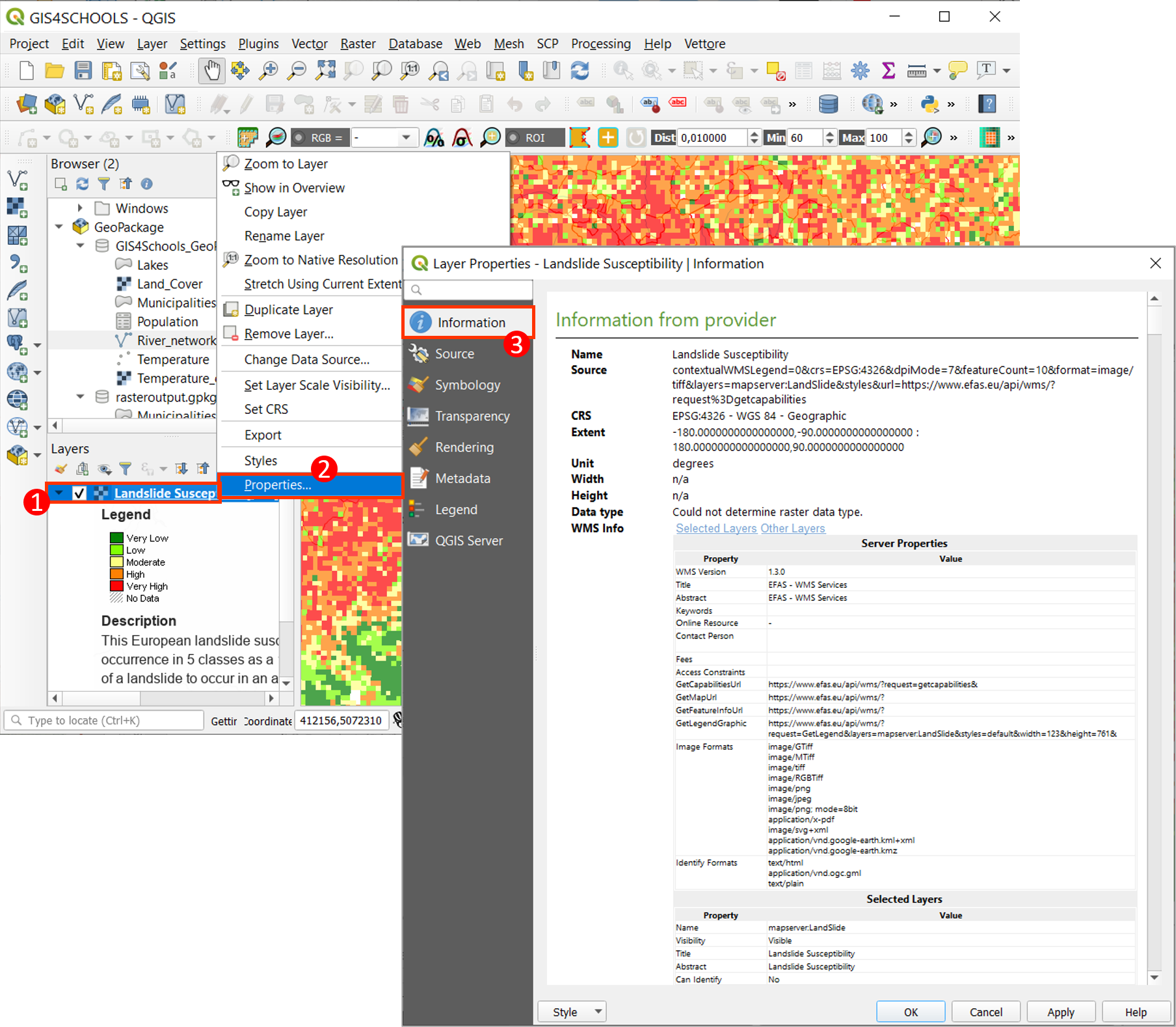
Fig. 2.2.1.3 – Analysing the Properties of the Landslide Susceptibility WMS layer
2.2.2. WFS
To add an OGC WFS layer, click on menu Layer (1) → Add Layer (2) → Add WFS Layer (3) (Fig. 2.2.2.1).
We upload data from the Network Services OGC of the Italian National Geoportal. Browsing the Geoportal we find the available WFS Services and we select Bacini idrografici principali e secondari. The URL of the service is http://wms.pcn.minambiente.it/ogc?map=/ms_ogc/wfs/Bacini_idrografici.map and then we can explore the capabilities of the service (XML file) by clicking on the Capability link. In order to add this WFS Service to QGIS, click New (4), name this layer Watershed (5) and copy the service URL (6). Click OK (7). Then click Connect (8): the service is providing two layers. We select the Bacini idrografici secondari layer (9) and we click Add (10). On the contrary to a WMS layer, a WFS layer is a real vector layer, i.e. we can see (query) all its properties (attribute table) and we can change the visualization style.
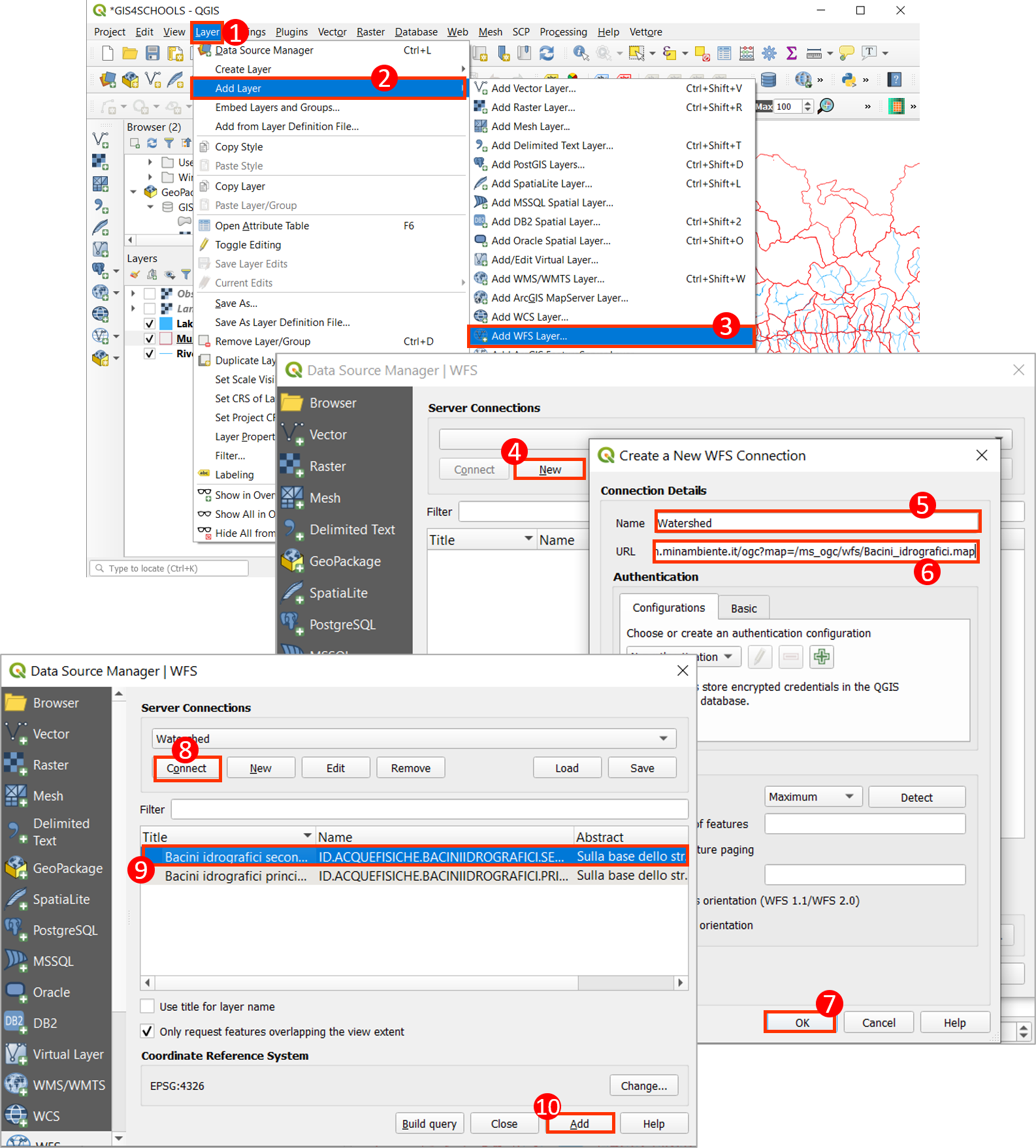
Fig. 2.2.2.1 – Adding a new WFS service (Bacini idrografici secondari layer)
We can customise the layer, for instance we can change its symbology (Fig. 2.2.2.2), changing the fill (1) and opacity (2). The result is visible in (3).
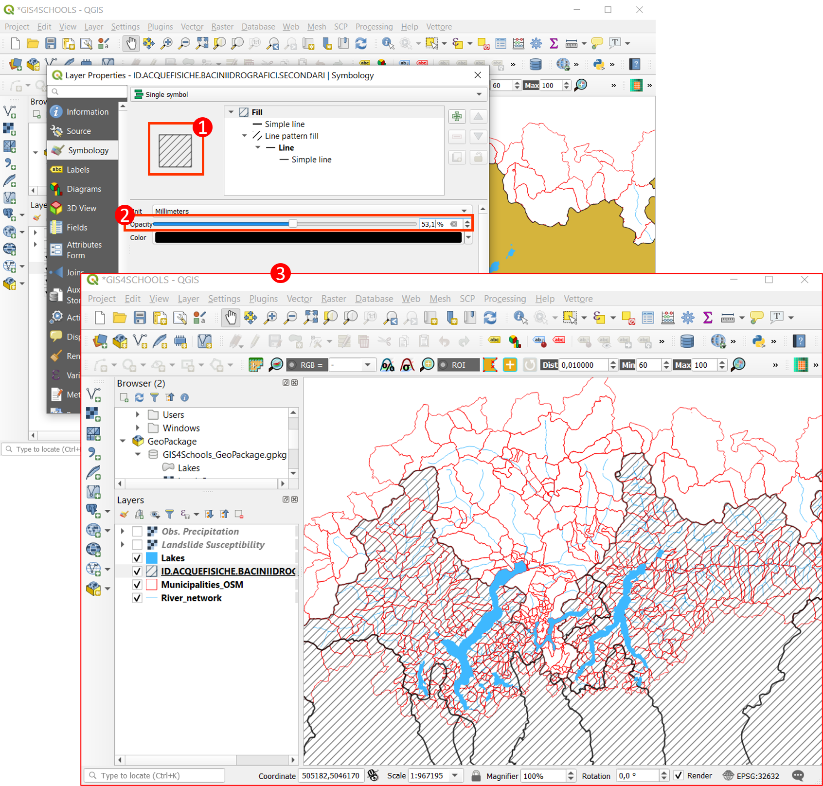
Fig. 2.2.2.2 – Changing symbology to the WFS Bacini idrografici secondari layer
Repeat what we have done, by connecting to the Catalogo frane (Landslide Catalogue) of the WFS Services of the Geoportal and connect to the Frane Poligonali layer. It will take a while for loading because the file is heavy and you can see the progression on a bar. Look at Fig. 2.2.2.3. The result is visible in Fig. 2.2.2.4.
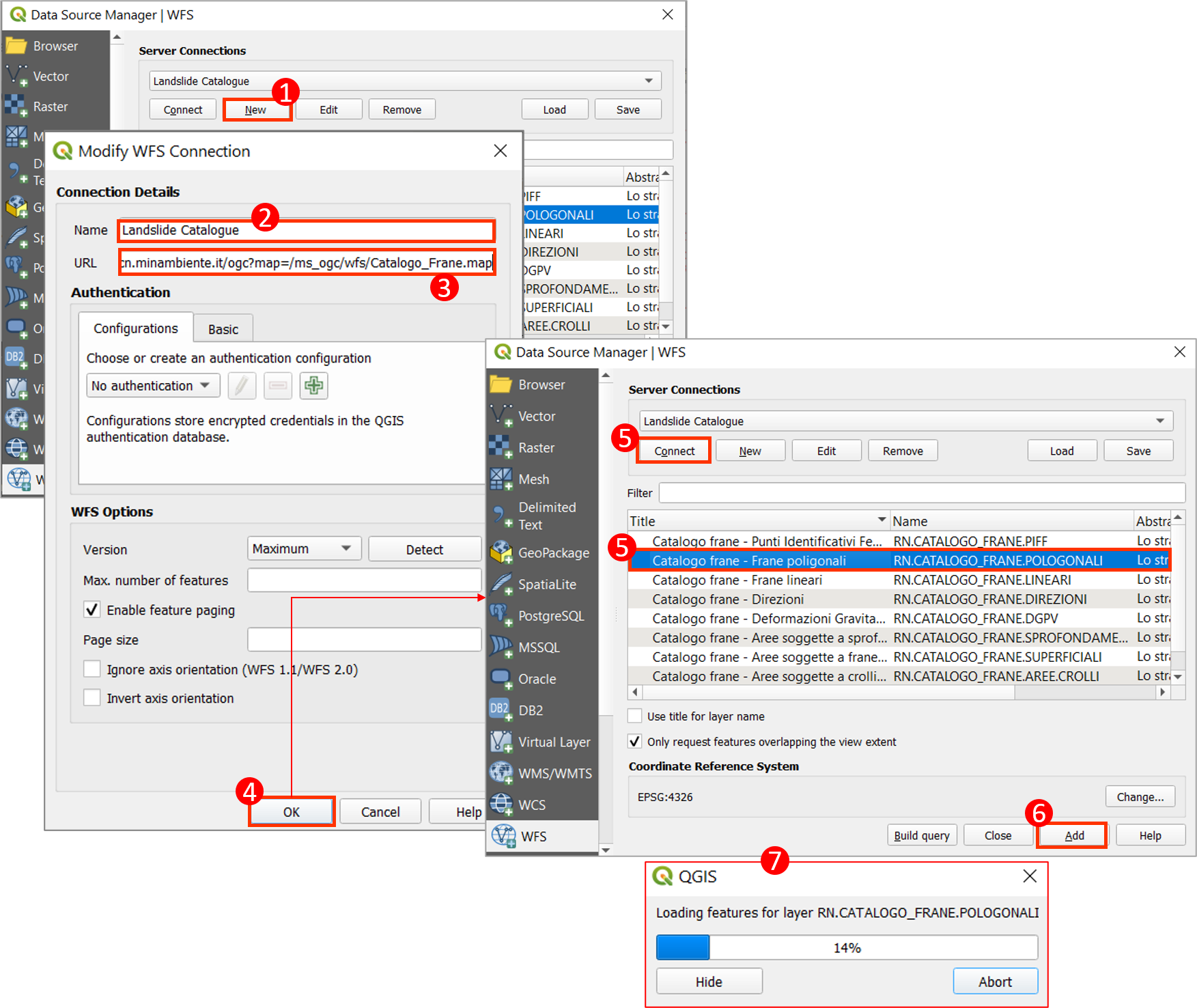
Fig. 2.2.2.3 – Connecting to the Catalogo_Frane WFS service and adding the Catalogo frane - Frane poligonali layer
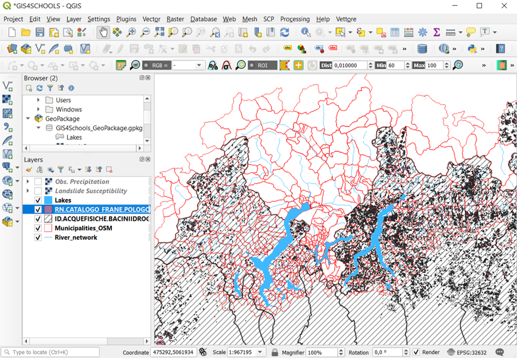
Fig. 2.2.2.4 – Visualization of the Catalogo frane - Frane poligonali layer
Now rename the two layers respectively as Watersheds and Polygonal Landslides, by right-clicking the layer and selecting Rename Layer. Look at Fig. 2.2.2.5 (1). A WFS layer cannot be edited directly, but it can be saved in a local system as a vector file and then we can create changes on the saved layer. Export the WFS Watersheds layer and save it in a local folder of your computer (Fig. 2.2.2.5). Right-click on the layer and select Export (2) → Save Features As (3). Save it as a shapefile (4) and give to this layer the name Watersheds_downloaded (5). Finally, click OK (6). You can visualise and analyse the new shapefile, for instance by opening the attribute table (Fig. 2.2.2.6). The advantage of having it in your local folder is that it will be always available, even if the server of the National Geoportal was not working or you had not the internet connection.The disadvantage is that you won’t have the updated layer if the service provider substitutes the layer with a new most updated one.
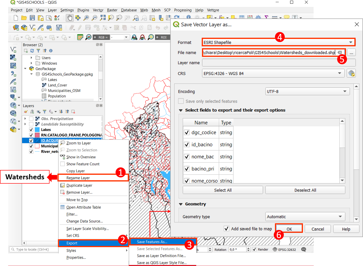
Fig. 2.2.2.5 – Rename a layer and export it as a shapefile
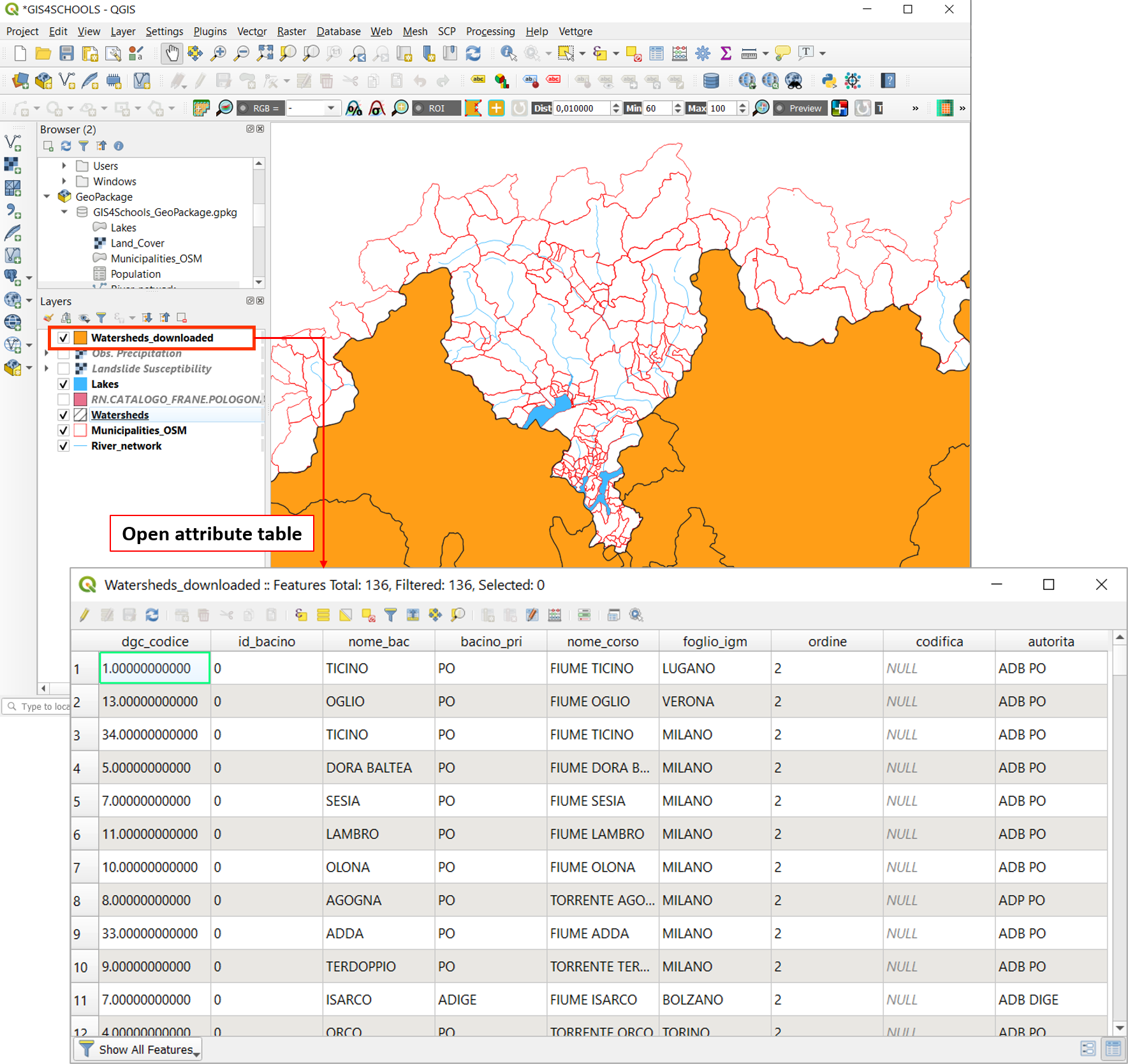
Fig. 2.2.2.6 – Visualization of the new shapefile (Watersheds_downloaded.shp), with its attribute table
2.2.3. WCS
To add an OGC WCS layer, click on menu Layer → Add Layer → Add WCS Layer.
We upload data from the Network Services OGC of the Italian National Geoportal. Browsing the Geoportal we find the available WCS Services and we select Modello digitale del terreno - 75 metri. The URL of the service is http://wms.pcn.minambiente.it/wcs/dtm_75m and we can explore the capabilities of the service (XML file) by clicking on the Capability link.
We add the service (1) (Fig. 2.2.3.1). We connect to the layer EL.DTM.75M, clicking on New (2). Name it DTM 75 m res (3) and copy the URL previously specified (4). Click OK and then Connect (5), select the layer EL.DTM.75M (6) and click Add (7). The result is visible in Fig. 2.2.3.1.
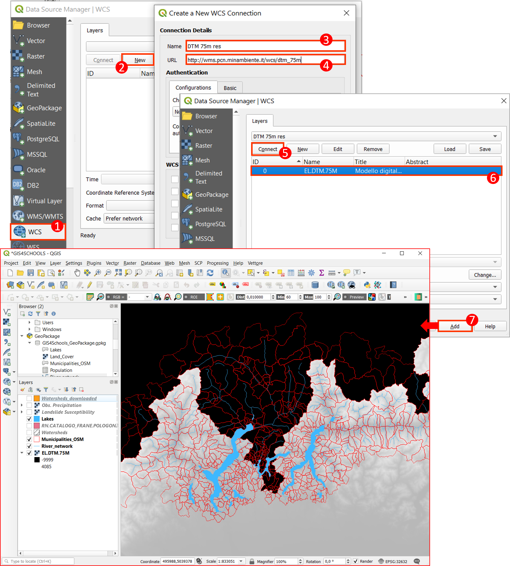
Fig. 2.2.3.1 – Connecting to the Modello digitale del terreno - 75 metri WCS service and adding the EL.DTM.75M layer
We can change the style of the layer, for instance using as rendering type the Hillshade obtaining the visualisation of Fig. 2.2.3.2 (upper part). As an alternative, select as render type the Singleband pseudocolor (Fig. 2.2.3.2, lower part). This flexibility is possible because the WCS is providing a raster file and not a simple image of the map as for the case of the WMS.
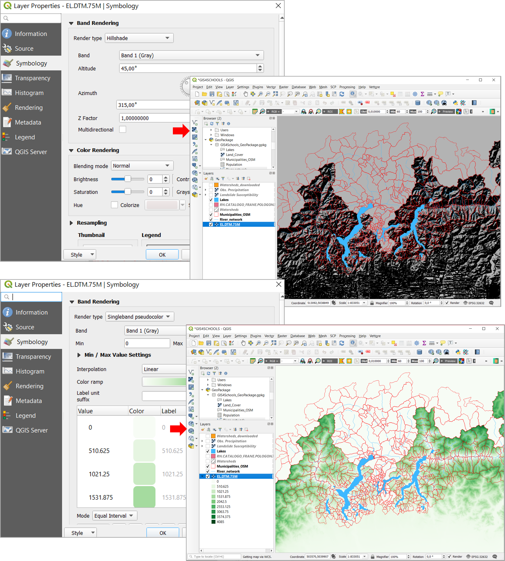
Fig. 2.2.3.2 – Changing symbology to the DTM 75 m res (WCS) layer: Hillshade (above) and Singleband pseudocolor (below) rendering
The raster data can be exported and saved in a local folder of your computer (Fig. 2.2.3.3). Right-click on the raster layer → Export (1) → Save As (2) and specify as file format GeoTIFF (3), assigning the name DTM_75m_res_downloaded (4). Click OK (5). The file is heavy and it requires a while. The advantage of having it in your local folder is that it will be always available, even if the server of the National Geoportal was not working or you had not the internet connection.The disadvantage is that you won’t have the updated layer if the service provider substitutes the layer with a new most updated one.
For appreciating the difference between a WCS and a WMS, connect to the WMS Network Services OGC of the Italian National Geoportal and select the Modello digitale del terreno - 75 metri. The URL of the service is http://wms.pcn.minambiente.it/ogc?map=/ms_ogc/WMS_v1.3/raster/DTM_75M.map and we can explore the capabilities of the service (XML file) by clicking on the Capability link.
Once you have connected to this service you can for instance compare what is possible in terms of change of symbology and visualisation. You will see that, on the contrary to a WMS layer, a WCS layer is a real raster layer and therefore visualization can be changed and values can be queried. However, its values cannot be edited directly , but it can be saved in a local system as a raster file and edited afterwards. By adjusting the values of extent while saving WCS we can choose which portion of it to save.
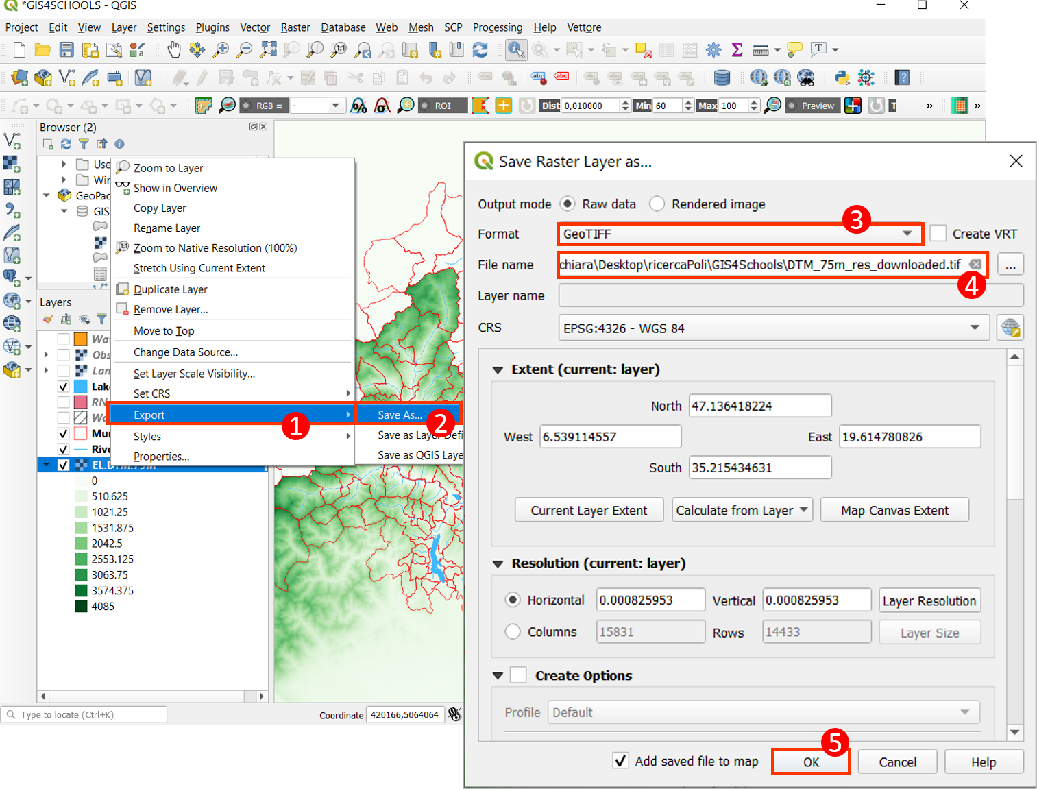
Fig. 2.2.3.3 – Exporting the DTM 75 m res (WCS) layer in the local directory
| [1] | European Commission, Joint Research Centre (2017): EFAS landslide susceptibility. European Commission, Joint Research Centre (JRC) [Dataset] PID: http://data.europa.eu/89h/3f7c3117-a72e-4e4e-bdec-f802e81e99a7 |
| [2] | European Commission, Joint Research Centre (2017): EFAS observed precipitation. European Commission, Joint Research Centre (JRC) [Dataset] PID: http://data.europa.eu/89h/e7db0ff2-e5c9-4006-9e24-30b98fe0f0f1 |